
Introduction
Workshop Synopsis:
This tutorial has been designed for a two-part full-day series of workshops at the University of Kent, which will provide students with an introduction to the Processing computer language. The first day you will be introduced to core programming terminologies, by coding basic programs, or sketches as they are referred to within Processing, demonstrating how programs are comprised of ‘syntax’, ‘functions’ and ‘data’ with a focus on how to draw 2D shapes. The first workshop will provide a foundation to move onto more advanced programming concepts. Click here to read the first workshop!
In the second workshop we will move towards three dimensions and learn how to make previously inanimate objects on a screen, interact with one another, act on individual rules and group behaviours, thus developing autonomous agents which can produce emergent ‘architectural’ forms. We will also briefly cover interaction with external data sources.
Workshop 2: Introducing Multiple Objects, 3D, Vectors and Agents
Workshop Two is a direct continuation of Workshop One: Learning Processing 3, if you’ve not followed from the beginning I would highly suggest you start with Workshop One, before continue to Workshop Two.
In this workshop we will extend what we’ve covered thus far to introduce more complex programming concepts such as arrays, which will allow us to create hundreds, even thousands of objects and we will no longer be confined to two dimensions as we will now explore how to draw in three dimensions. From here we will introduce vectors and forces which will form the foundation of calculating the motion of objects know as agents, which interact with one another as they move through space.
1. Arrays: Many Elements
The first lesson of Workshop Two will introduce a new core programming terminology and concept know as arrays. We will use arrays to extend the final Processing Sketch we developed in Workshop One, in which we constructed a class which describes a box.
Within Processing there are two principle types of arrays: fixed length arrays and variable length arrays, to begin we will investigate the former and some permutations of fixed length arrays such as first for lists and for lists. After that we will move to variable length arrays which will allow us to add arbitrary number of boxes to the canvas, without us having to repeat code unnecessarily.
Following this we will introduce dynamic motion in the form of a simulated gravitational field, facilitating our rotating boxes to ‘orbit’ around one another.
Key programming concepts:
Arrays, ArrayLists, enhanced loops and classes
1.1 Introduction
Following on from Workshop One’s last lesson: Introducing Classes (OOP) where we finally gained full control over each of our boxes and where each box was truly independent from one another, we will now look at solving a remaining limitation of that sketch, which was the limited number of boxes which we could create, without duplicating code. To create another box we needed to add code: each box required a call to its: ‘constructor’, ‘draw’ and ‘mousePressed’ function. Suppose we need 30 boxes this would require 30 lines of code multiplied by 3, or a total of 90 new lines. To solve this, would it not be simpler have a list of some sort to store each box and then be able to tell Processing once to call the ‘draw‘ function for all the boxes in said list. For this, there are arrays. We can iterate through the array, and access each element by integer position, from 0 to how ever many elements there are in the array. One important point to note, is that all arrays usually start from 0, or in other words the ‘data’ contained at the beginning of the array is at position (index) 0, this is one of the reasons we start ‘for‘ loops from 0.
By using arrays we can in fact have boxes which interact with other boxes, by passing array members (in this case boxes) to each other as a parameter. We will do just this to create a gravitational attraction, between each and every box.
1.2 Fixed Length Arrays
You can think of an array essentially as a list, which can be cycled through — therefore we can store a series of data elements as a single name: shoppingList: pasta, tomatoes, zucchini, eggs, potatoes, beer, etc…
A ‘for‘ loop will be used to cycle through each array element in sequence and an element can be accessed by referring to its position (index) within the list. Take the above shoppingList as an example, if I wanted to refer to eggs I would refer to its index: 3. Later, I will also introduce a new type of ‘for‘ loop, know as an ‘advanced for loop’ which is useful when we want to make reference to a single element within an array.
Using an array will also simplify drawing, as you don’t need to write the parameters for each rectangle and apply whatever function we want to make the rectangle do something every time, thus making the processes of coding easier or at least reducing how much code we need to write.
1.2.1 Fixed Length Arrays Of Integers
Lets look at the following task: create 10 squares of different sizes and display them on the canvas. We can use an array when we have a list of information. To solve this task we could write the following in Processing:
rect(0,0,10,10);
translate(10,0);
rect(0,0,5,5);
translate(10,0);
rect(0,0,3,3);
translate(10,0);
rect(0,0,2,2);
translate(10,0);
rect(0,0,11,11);
translate(10,0);
rect(0,0,6,6);
translate(10,0);
rect(0,0,8,8);
translate(10,0);
rect(0,0,11,11);
translate(10,0);
rect(0,0,4,4);
translate(10,0);
rect(0,0,9,9);
translate(10,0);
As you can see there is a sizeable amount of repetition in the above code. It would be better if we could create a list of 10 different square sizes, and then draw the squares using a loop.
We can proceed as so, firstly we need some code to define our array of square sizes:
int[] x = {10,5,3,2,11,6,8,11,4,9};
Index |
0 | 1 | 2 | 3 | 4 | 5 | 6 | 7 | 8 | 9 |
Element |
10 | 5 | 3 | 2 | 11 | 6 | 8 | 11 | 4 | 9 |
Let’s analyse the above syntax. The ‘int[]‘, declares this as an array (‘[]‘) of type integers. The ‘=‘ immediately assigns the array with a list, which is specified using curly brackets. Notice the differences between this and a straight declaration of an integer: int x = 3; and int[] x = {0,1,2,3};. We can access an element within the array by using the index of that element. We start by counting at 0, so the 0’th element in ‘squaresizes’ is 10, the 1’st is 5 and so forth. To obtain an element from the array in Processing, we make use of square bracket notation. For example, to draw the first square in the list, we would write:
int[] x = {10,5,3,2,11,6,8,11,4,9};      // Declar an integer type array with the following integers
rect(0,0,x[0],x[0]);                     // Draw a rectangle at {0,0} with size of the 0th index value in the array (10)
We can also mix array elements by using alternative index, for example to make a thin tall rectangle:
int[] x = {10,5,3,2,11,6,8,11,4,9};      // Declar an integer type array with the following integers
rect(0,0,x[2],x[4]);                     // Draw a rectangle at {0,0} with width 2nd index value (3) and height 4th index value (11)
Notice how we write the variable name ‘x‘ followed by the index of the element we want contained between square ‘[]‘ brackets. We don’t have to use a constant value between the square brackets either, we could in fact use another variable. This is how we will combine a ‘for‘ loop with our array to draw 10 boxes using the sizes we’ve specified in the array. Our loop index ‘i‘ will begin at 0, as usual, and count to 9, as so:
int[] x = {10,5,3,2,11,6,8,11,4,9};      // Declar an integer type array with the following integers
for (int i=0; i < 10; i++){              // Loop 10 times
  rect(0,0,x[i],x[i]);                   // Draw a rectangle at {0,0} with width 'i' as the index
  translate(10,0);                       // Each loop: translate 10 pixels to right
}
Notice in the above how we’ve reduced out initial code from 20 lines down to 5 lines of code. Also don’t forget that for each loop we need to include the ‘translate‘ function to cumulatively shift each box 10 pixels to the right.
In addition to allowing us to access different elements in the array, arrays (like String) have some special data associated with them. One you will frequently make use of is ‘length‘. These can be accessed using the dot notation, just as we would for class member functions and variables. The array ‘length’ is a query-type function and returns the length (or how many elements are in the array). To use ‘length()‘ we append it to the name of our array variable, as so: ‘x.length‘.
We can update our code to use the array length to determine how many times our loop should occur, which further allows us to change how many elements we include in the array. For example:
int[] x = {10,9,3,2,11};              // Declar an integer type array with the following integers
for (int i=0; i < x.length; i++){     // Loop as many times as there are elements in the array
  rect(0,0,x[i],x[i]);                // Draw a rectangle at {0,0} with width 'i' as the index
  translate(10,0);                    // Each loop: translate 10 pixels to right
}
Notice how the above code works. The loop counts from 0 up till the value which ‘x.length‘ returns, in our case 5, less one due to the less-than operator. Our array has 5 elements, so the loop counts from 0 to 4, ensuring each element of the array is drawn on the canvas.
1.2.2 Fixed Length Arrays Of Classes
We are not only limited to arrays which contain integer elements. Like any variable, we can create arrays which store any type, or, better yet any class. Therefore, if we need to create an array of boxes, we can use a similar syntax.
Firstly, we will need the the rotating box class from the previous workshop. I’ve included the code bellow, which you can copy and past into Processing. Note there are some minor alterations to the code allowing us to pass even more parameters than before, see lines 15 and 16:
/*
    * Learning Processing 3 Intermediate - Lesson 1: Arrays: Many Elements
 *
 * Description: Basic example of implementing a class within Processing and an ArrayLists of Classes
 *
 * © Jeremy Paton (2018)
 */

//Objects/Classes
Box box1, box2;

void setup() {
  size(400, 400);
  rectMode(CENTER);                                        // Set rectangle to draw from its centre
  box1 = new Box(width/2, height/2, 20, 0.8, true);        // Construct box1 with parameters (posX, posY, size, speed, spinning)
  box2 = new Box(width/2+50, height/2-50, 60, 0.3, true);  // Construct box2 with parameters (posX, posY, size, speed, spinning)
}

void draw() {
  background(39, 40, 34);                       // Redraw the background
  box1.draw();                                  // Draw box1
  box2.draw();                                  // Draw box2
}

void mousePressed() {                           // Special function used for 'listening' for a mouse press
  box1.mousePressed();                          // Call box1's mousePressed function
  box2.mousePressed();                          // Call box1's mousePressed function
}
/*
* Class: a Box (literally just a box!)
*
* Description: Above ^
*
* @param {int} frame - increasing counter based on frameRate();
* @param {float} posX - x coordinate for the centre of the rectangle
* @param {float} posY - y coordinate for the centre of the rectangle
* @param {float} side - size of the box
* @param {float} rps - revolutions per second (mapped between 0 deg and 20 deg)
* @param {boolean} spinning - on/off toggle
*/
class Box {
// Class Variables
int frame = 0; // Declare integer type GLOBAL variable and assign it the value 0
float posX; // Declare float type GLOBAL variable for x-position of box
float posY; // Declare float type GLOBAL variable for y-position of box
float side; // Declare float type GLOBAL variable for size of box
float speed; // Declare float type GLOBAL variable for speed of box rotation
boolean spinning; // Declare boolean type GLOBAL variable and assign it true
//Constructor
Box(float x, float y, float s, float rps, boolean spin) {
posX = x; // Set posX equal to the parameter x
posY = y; // Set posY equal to the parameter y
side = s; // Set side equal to the parameter s
speed = map(rps,0,1,0,0.35); // Set speed equal to (mapped between 0 deg and 20 deg)
spinning = spin; // Set spinning state equal to the parameter spin
}
void draw() {
pushMatrix(); // Save global coordinate frame
translate(posX, posY); // Translate coordinate frame to posX and posY
rotate(speed * frame); // Rotate by x deg, each frame
rect(0, 0, side, side); // Draw rect, with position at origin and a size of side
popMatrix(); // Restore global coordinate frame
if (spinning) { // If 'spinning' is true continue
frame++; // Increment our frame counting variable by 1
}
}
void mousePressed() { // Special function used for 'listening' for a mouse press
if (dist(mouseX, mouseY, posX, posY) <= side/2) { // If the distance between the mouse and center is (less or equal) the radius
spinning = !spinning; // Set spinning equal to the inverse of spinning's existing value
}
}
}We’re now going to focus on the Main Code tab and instead of initialising each box one at a time, each with their own variable, we can list each box within an array as we’ve done previously with integers:
Box[] boxes = {new Box(width/2, height/2, 20, 0.8, true), new Box(width/2+50, height/2-50, 60, 0.3, true)};Whilst the above line looks rather intimating, it’s actually no more difficult than what we’ve already seen. The method to construct each new box in the list is exactly as it was in the last Workshop: each box must be declared as a ‘new’ instance of the Box class and each one has five parameters (x, y, size, spin speed and spin state). This list of new boxes is then encapsulated between braces ‘{‘ and ‘}‘, and the declaration changed to indicate that the array is of type Box (‘Box[]‘) rather than for a singular Box.
We may encounter situations where we needing to assign the elements of our array within the ‘setup‘ function, rather than as part of a global variable. In order to do so we need to write the following:
Box[] boxes;                                    // Declare an array variable as type Box
void setup() {
  size(400, 400);
  rectMode(CENTER);
  // Assign boxes with two instance of our box class
  boxes = new Box[]{new Box(width/2, height/2, 20, 0.8, true), new Box(width/2-40, height/2+50, 50, 0.2, true)};
}
Notice the difference between declaring and assigning the ‘boxes‘ array in a single line compared to assigning the elements to it within ‘setup‘. We firstly define the variable (array) we will assign the boxes to using ‘=‘, followed by ‘new Box[]‘ and lastly we encapsulate the list of new boxes between curly brackets.
Now that we’ve setup our array to contain two boxes, we can use it in the same way we have previously used an integer array, as so:
void draw() {
  background(39, 40, 34);                       // Redraw the background
  for (int i=0; i < boxes.length; i++){         // loop for length of boxes array
    boxes[i].draw();                            // Call box draw function
  }
}

void mousePressed() {                           // Special function used for 'listening' for a mouse press
  for (int i=0; i < boxes.length; i++){         // loop for length of boxes array
    boxes[i].mousePressed();                    // Call box mousePressed function
  }
}
1.3 ‘Variably‘ Fixed Length Arrays
While in some cases you know beforehand what the data you require is prior to writing your code (as was demonstrated in the array of squares), in most cases you do not (for example, if you are loading in many shapes from a file). Furthermore, you may not even know how many items you want in your array before you start.
In order to demonstrate this lets change the declaration of the ‘boxes‘ array at the start of your sketch:
Box[] boxes = new Box[30]; // Declare an array with 30 EMPTY Box objectsAlso make sure to comment out the following line, temporarily, which will help to demonstrate more accurately what the new array declaration code above actually does:
// boxes = new Box[]{new Box(width/2, height/2, 20, 0.8, true), new Box(width/2-40, height/2+50, 50, 0.2, true)};Note that ‘new Box[30]‘ does not create any boxes, it simply tells Processing that the ‘boxes‘ array should contain 30 slots for Box type elements. If you run the sketch now it will crash, generating the following error:
Null Pointer Exception
This is most likely your first encounter of a memory error. Until now, every error we’ve encountered will have been a syntactic error. That is, a typo, a call to a function misspelled and so on. A memory error is a different, and a far more nefarious error. The syntax of the sketch as it stands is perfect, but because we have only created an empty list (series of containers) to place Box objects into, rather than the Box objects themselves, when we come to use them, in the ‘draw‘ function and the ‘mosuePressed‘ function, Processing finds a nothing object, a ‘null’, and it crashes. The problem with memory errors is that they can be very difficult to find: we may forget to initialise boxes but only use them many lines later. Notice how the above ‘Null Pointer Exception’ provides no indication of where the error occurred, therefore, finding out what went wrong can be very tricky.
That’s the gist of memory errors, just remember the ‘Null Pointer Exception’ as a clue that you have a memory error (usually a variable or array which has not been assigned any ‘data’ before it was used). Now let us move onto fixing this problem. We’ve stated that the array should contain 30 elements, thus we need to create 30 new boxes to fill our array. In order to achieve this, we change the ‘setup‘ function. Note, it must be the ‘setup‘ function in order that the boxes are initialised before they are used in the ‘draw‘ function.
The initialisation code will now look like this:
void setup() {
  size(400, 400);
  rectMode(CENTER);
  // loop for length of array (30)
  for (int i=0; i < boxes.length; i++){
    // each loop - create a new box with randomised parameters
    boxes[i] = new Box(random(width), random(height), random(5, 25), random(1), randomBoolean());
  }
}
I have used a function we’ve not used often before, ‘random‘. When called with a single parameter, as in the ‘random(width)‘ the function creates a random floating point number between 0.0 and 100.0. The two calls to ‘random(width)‘ and ‘random(height)‘ create (different) random x and y coordinates for each box. Next, when ‘random‘ is called with two parameters, as in random(5, 25), it generates a random float from 5.0 to 25.0. I’ve used this so we only get boxes of a reasonable size: larger than 5 pixels yet, smaller than 25 pixels. Lastly to create a random boolean (true of false) to control the spinning state of the box, I’ve created my own function: ‘randomBoolean‘. Processing unfortunately has no shortcut method to create a random boolean, therefore we need to write this logic ourselves and encapsulate it within a function. This is also the first example, of a custom function which returns a value, which we’ve encountered so far.
The code for our ‘randomBoolean’ function is as follows:
boolean randomBoolean() {
  return random(1) < 0.5;         // If random float is larger than 0.5 return true (50% probability)
}
Our ‘randomBoolean’ function won’t require any parameters, but it needs to return either a true or false value. To do this we remove the word ‘void‘ from the beginning of the function name and replace it with ‘boolean‘ which indicates that the type of data which the function will return is a boolean. Inside of our function we can write our logic in a single line, which is similar to the probability code we wrote in Workshop One: 3.8 Code Challenge (10PRINT). We simply tell processing to ‘return‘ the result of the condition ‘random(1) < 0.5‘. This results in a 50% probability of either a true or false value being returned.
There is an argument, that for every call to the ‘randomBoolean’ function we should first randomise the probability before the condition statement, thus for each call the probability won’t always be 50% and therefore our randomisation is more random. However, this is not particularly necessary right now.
We can of course also use a variable to set the size of the array when we declare it:
int noOfBoxes = 30;                            // Declare an interger variable with the value 30
Box[] boxes = new Box[noOfBoxes];              // Declare an array with size of 'noOfBoxes'
1.4 Variable Length Arrays: ArrayLists
Before we proceed I need to introduce a completely new type of array, known as an ‘ArrayList‘. Whilst the previous ‘fixed length arrays‘ (standard ‘array‘) are useful, as we start exploring more complex projects involving many objects and in which we are constantly adding and removing objects (hence adding and removing elements of an array), fixed length arrays will cause more challenges, which can be negated by using the more flexible ‘ArrayList‘.
In essence an ArrayList stores a variable number of objects. This is similar to making a standard array of objects, however, with an ArrayList, items can be easily added and removed from the ArrayList and it is resized dynamically. This will prove very convenient, though it’s slower than making an array of objects when using many elements, but, more suited towards arrays containing classes-objects, such as our Box class, as it has many methods used to control and search its contents. These include:
- size() method — used to get the length of the ArrayList, returned as an integer value for the total number of elements in the list.
- add() method — used to add an element to ArrayList, added at the end of the array by default.
- remove() method — used to remove an element from an ArrayList.
- get() method — used to return an element at the specified position in an ArrayList.
We are now going to convert our code from using a standard array to an ArrayList, from here we will include a function which allows us to add rotating boxes by clicking on the canvas. Firstly we need to change the declaration from a standard array to an ArrayList, which can be achieved as follows:
ArrayList<Box> boxes = new ArrayList<Box>(); // Declare an ArrayList of type BoxLet’s take a look at the syntax of the code above in order to determine what each part means. Firstly we write ‘ArrayList‘, which tells Processing that we are declaring an ArrayList, and takes the place of our previously used square brackets ‘[]‘ which indicated that we were creating a standard array. Also note that we write ‘ArrayList‘ at the start rather than after the type declaration. Next we tell Processing what type of data the ‘ArrayList‘ will contain, in this case ‘Box‘, this is written immediately after ‘ArrayList‘ and is contained within angle brackets ‘<‘ and ‘>‘. So what we’ve currently instructed Processing to do is create an ArrayList which accepts elements which are of the type ‘Box‘: ArrayList<Box> boxes.
Next, we are going to assign the ‘ArrayList‘ with data and a size. However, we don’t have the data ready nor do we know how many elements our ‘ArrayList‘ will need to store, therefore, we will tell Processing to store a ‘placeholder-like’ value in the ‘ArrayList‘ and that the ‘ArrayList‘ has no starting capacity, it is empty. This is done by assigning the ‘ArrayList‘ as follows: = new ArrayList<Box>();
This can be expressed as the follow: ArrayList<Type> boxes = new ArrayList<Type>(InitialCapacity);
Now we need to modify the code within ‘setup‘ to work with an ArrayList rather than a standard array, we can do this by making the following changes:
void setup() {
  size(400, 400);
  rectMode(CENTER);
  // loop for as many boxes as we want created (30)
  for (int i=0; i < 30; i++){
    // each loop - create a new box with randomised parameters and add it to the ArrayList
    boxes.add(new Box(random(width), random(height), random(5, 25), random(1), randomBoolean()));
  }
}
Take a look at line 7: here we’ve made a change to our code to make use of one of the special methods associated with ArrayLists, in this case the ‘add‘ function. We first write the name of the ArrayList variable ‘boxes‘ and then using dot notation (as ArrayList is actually a class), we call the ArrayList ‘add‘ function, which requires a parameter, and in this case it can be any ‘Box‘ type object, which is encased in round brackets. That’s most of the changes for the ‘setup‘ function, however, as the ‘boxes‘ ArrayList was declared as empty we can no longer use the size of the array to loop, and need to change this back to a constant value or an integer variable, see line 5.
Let’s now focus on the ‘draw‘ function and ‘mousePressed‘ function and make the changes necessary to update our code to work with an ArrayList. Here we are going to need to use the ArrayList ‘get‘ function, as so:
void draw() {
  background(39, 40, 34);                       // Redraw the background
  for (int i=0; i < boxes.size(); i++){         // loop for length of boxes array
    boxes.get(i).draw();                        // Call box draw function
  }
}

void mousePressed() {                           // Special function used for 'listening' for a mouse press
  for (int i=0; i < boxes.size(); i++){         // loop for length of boxes array
    boxes.get(i).mousePressed();                // Call box mousePressed function
  }
}
Firstly we’ve needed to update our loop to get the size (length) of our ‘boxes‘ ArrayList, on lines 3 and 9. Unlike a standard array where we use ‘length‘ which acts more like a variable, ArrayLists require us to use ‘size()‘, which is a question-style function and returns an integer value, in our case the number of elements within the ‘boxes‘ ArrayList (30). Next we change lines 4 and 10 to use the ‘get‘ function by writing the name of the ArrayList variable ‘boxes‘ and then using dot notation we call the ArrayList ‘get‘ function, which requires a parameter which is the index (position) of the element in the ArrayList. This is similar to how we previously included the index of the array within square brackets. Then we follow this by another dot notation which we call the ‘draw‘ and ‘mousePressed‘ functions of the particular box stored in the ‘i‘ index of the ArrayList.
We’ve now successfully converted our code to use an ArrayList, before we progress I want to quickly introduce a new type of loop, which is referred to as an ‘enhanced for loop’.
1.5 ArrayLists: A Case For Using Enhanced Loops
Enhanced Loops simplify the syntax of a standard ‘for‘ loop by removing the need to declare a counter variable ‘i‘, a condition statement ‘i < x‘ and a increment operator ‘i++‘. Enhanced loops also remove the requirement to use the ‘get‘ function associated with an ArrayList as this process is built into the syntax of the enhanced loop, and thus helps us to write condensed code. Enhanced loops and ArrayList go hand in hand and are to use an enhanced loop you need to be looping through an ArrayList.
We are now going to change the ‘draw‘ and ‘mousePressed‘ functions to use enhanced loops, instead of traditional ‘for‘ loops, as follows:
void draw() {
  background(39, 40, 34);        // Redraw the background
  for (Box b: boxes) {           // Enhanced loop through ALL elements of boxes AS b
    b.draw();                    // Call box mousePressed function
  }
}

void mousePressed() {            // Special function used for 'listening' for a mouse press
  for (Box b: boxes) {           // Enhanced loop through ALL elements of boxes AS b
    b.mousePressed();            // Call box mousePressed function
  }
}
If we analyse the code above, specifically lines 3 – 4 and lines 9 – 10, you will see how we write an enhanced loop. We still write ‘for‘, however, our loop parameters are vastly different. What we are in fact telling Processing to do is loop through all elements of the ‘boxes’ ArrayList, and for each loop store the element (object) contained in the ArrayList in the variable ‘b‘. This can be expressed as follows:
for (type element: array)
The enhanced loop starts from the first element in the ArrayList ‘0‘ and iterates to the last ‘n‘, always from beginning to end. For each iteration of our enhanced loop we ‘get‘ the element (class-object) at the index of that iteration and assign this element of the array to a variable we’ve declared called say ‘b‘, which we have told Processing is a Box type variable. The variable type declared within the enhanced loop must mach the type we’ve defined the ArrayList as containing.
Limitations of using an enhanced loop:
Whilst an enhanced loop simplifies the code and streamlines it, it is not always a workable solution and here are some limitations regarding the use of an enhanced loop. Firstly they always iterate from start to end, thus if we need to loop backwards through the array we can’t use an enhanced loop. Secondly, an enhanced loop will always iterate through the entire array, thus if we need to stop iterating, say half way, we cannot.
1.6 User Interaction: Dynamically Adding To An ArrayLists
We mentioned earlier that once we’ve converted our code to use an ArrayList we would add functionality allowing us to add rotating boxes by clicking on the canvas. However, I want to maintain the functionality which allows us to stop and start a box from rotating by also clicking on it. Thus adding more rotating boxes will not be as simple as it may have previously seemed. To solve this we are going to employ much of what we’ve covered thus far.
First lets identify a fundamental problem if we add a rotating box by clicking on the canvas. Which is what would happen if we clicked on top of an exiting box? Will this stop that box and not create a new box or will a new box appear above the box we clicked on and impede us from interacting with the box underneath the new box.
Therefore, I propose that we need to first check if we’ve clicked on an existing box. If we have then that box will stop or start spinning, but a new box will not be created. Alternatively when we click on the canvas if we’ve not clicked on an existing box a new box will be created at the location of our mouse cursor.
To do this we need to make a change to the ‘mousePressed‘ function in the ‘Box‘ class, which will let us know if we have in fact clicked on an existing box, we can do this as so:
boolean mousePressed() {                                // Special function used for 'listening' for a mouse press will return a boolen
  if (dist(mouseX, mouseY, posX, posY) <= side/2) {     // If the distance between the mouse and center is (less or equal) the radius
    spinning = !spinning;                               // Set spinning equal to the inverse of spinning's existing value
    return true;                                        // Return true - i.e we clicked this box
  } else {
    return false;                                       // Return false - i.e we did not clicked this box
  }
}
As we’ve done earlier for the ‘randomBoolean‘ function we have changed the ‘mousePressed‘ function in the ‘Box‘ class to return a boolean value. This will be used within the main sketch ‘mousePressed‘ function to know if we’ve clicked on an existing box. The ‘Box‘ class’s ‘mousePressed‘ function will return true when the distance between the mouse and the box is less than the size of the box divided by 2, which indicates the mouse did click a box. Else we return false, which indicates the mouse did not click a box.
When we specify that a function returns a value it’s important to make sure that the function in question will always return a value. When using an ‘if‘ statement to determine the return value it may be possible that the return value is not calculated as if the ‘if‘ statement resolved false it may skip the return line. Hence it is necessary to include an ‘else‘ statement at the end to insure that return is assigned a value. Processing will often notify you if it thinks a function which should return a value may not have an accessible return.
Now we need to return to the Main sketch tab to make the final changes, which will use the returned boolean value from the ‘Box‘ class’s ‘mousePressed‘ function, to determine whether a new box should be created or a whether an existing box was clicked. The changes are as follows, within the main ‘mousePressed‘ function:
void mousePressed() {            // Special function used for 'listening' for a mouse press
  boolean check = false;         // Declare a boolean variable with the value false
  for (Box b: boxes) {           // Enhanced loop through ALL elements of boxes AS b
    if (b.mousePressed()) {      // Call box mousePressed function
      check = true;              // If mousePressed returned true, set the check variable to true
    }
  }
  if (!check) {                  // If the checked variable is still false (i.e. no boxes were clicked on)
    // Add a box at the mouse cursors location to the ArrayList
    boxes.add(new Box(mouseX, mouseY, random(5, 25), random(1), randomBoolean()));
  }
}
We first need to declare a boolean variable within the ‘mousePressed‘ function and assign it the value true. Each time we call the ‘mousePressed‘ function (every mouse click) this variable will start with the value true. We will call this variable ‘check‘ on line 2. Next we need to alter the code within the enhanced loop by including the call to the class’s ‘mousePressed’ function as part of an ‘if‘ statement’s condition. We’ve done this on line 4, when we call the class’s ‘mousePressed’ function it will return a true or false value based on whether we did click this particular box. If the class’s ‘mousePressed’ function returns true, our if statement resolves to true and we proceed onto the next line, line 5. On line 5 we change the value of ‘check‘ to true. It’s important to note that we are looping through all the boxes in the ArrayList, and for a single mouse press we most likely would click on one of those boxes (not all of them) or non of them, hence our ‘check‘ variable acts like a gate, if for any of the boxes we loop through returns true we must have clicked on at least one box. It does not matter which box, just that we’ve clicked on one!
We now include a new ‘if‘ statement outside the enhanced loop which checks what the final value of the ‘check‘ variable is after looping through all the box’s ‘mousePressed’ functions, see line 8. If it is false (no boxes clicked), our ‘if‘ statement resolves to true as we’ve inverted the checked value using a ‘not‘ operator. Thus we progress to the next line, line 10. Line 10 uses the special ArrayList ‘add‘ function to add a new box to the end of the ArrayList, we no longer pass a random position for the box, but rather the mouseX and mouseY position.
If during the enhanced loop one of the box’s ‘mousePressed’ functions returned true, we would have set the ‘check‘ variable to true and therefore the ‘if‘ statement on line 8 would resolve to false, and skip line 10. Hence no box is added, as the mouse click was over an existing box’s position and intended to stop that box or start it from spinning.
1.7 Gravitational Fields
For a little fun, let us try a more involved sketch than we have produced so far.
First, we need to make some extensions to the variables which define the properties of our Box class. We will add two variables called ‘movX’ and ‘movY’ for the x and y component of the velocity to apply to the Box class:
class Box {

  // Class Variables
  int frame = 0;                   // Declare integer type GLOBAL variable and assign it the value 0
  float posX;                      // Declare float type GLOBAL variable for x-position of box
  float posY;                      // Declare float type GLOBAL variable for y-position of box
  float movX;                      // Declare float type GLOBAL variable for x-component of the velocity
  float movY;                      // Declare float type GLOBAL variable for y-component of the velocity
  float side;                      // Declare float type GLOBAL variable for size of box
  float speed;                     // Declare float type GLOBAL variable for speed of box rotation
  boolean spinning;                // Declare boolean type GLOBAL variable and assign it true

  //Constructor
  Box(float x, float y, float s, float rps, boolean spin) {
    posX = x;                      // Set posX equal to the parameter x
    posY = y;                      // Set posY equal to the parameter y
    side = s;                      // Set side equal to the parameter s
    speed = map(rps,0,1,0,0.35);   // Set speed equal to (mapped between 0 deg and 20 deg)
    spinning = spin;               // Set spinning state equal to the parameter spin
    movX = random(-1,1);           // Assign a random x component velocity between -1 & 1
    movY = random(-1,1);           // Assign a random y component velocity between -1 & 1
  }

  void draw() {
    posX += movX;                     // Increase the x position of the box by movX
    posY += movY;                     // Increase the y position of the box by movY
    pushMatrix();                     // Save global coordinate frame
      translate(posX, posY);            // Translate coordinate frame to posX and posY
      rotate(speed * frame);            // Rotate by x deg, each frame
      rect(0, 0, side, side);           // Draw rect, with position at origin and a size of side
    popMatrix();                      // Restore global coordinate frame
    if (spinning) {                   // If 'spinning' is true continue
      frame++;                        // Increment our frame counting variable by 1
    }
  }

  boolean mousePressed() {                                // Special function used for 'listening' for a mouse press will return a boolen
    if (dist(mouseX, mouseY, posX, posY) <= side/2) {     // If the distance between the mouse and center is (less or equal) the radius
      spinning = !spinning;                               // Set spinning equal to the inverse of spinning's existing value
      return true;                                        // Return true - i.e we clicked this box
    } else {
      return false;                                       // Return false - i.e we did not clicked this box
    }
  }
}
Once you’ve made the necessary changes, by assigning the new ‘movX‘ and ‘movY‘ variables with a random floating point number between (-1 and 1), line 20 and 21, followed by increasing the Box’s x and y position for each frame by ‘movX‘ and ‘movY‘, lines 25 and 26, you can run the sketch. Now you will see that the boxes should disappear off the canvas, as, at each call to each box’s ‘draw‘ function, it adds the value of ‘movX‘ to ‘posX‘, and similarly the value of ‘movY‘ to ‘posY‘. The variable ‘movX‘ and ‘movY‘ are assigned values just once, both within the Box constructor. The constructor for each box is called only once, from the ‘setup‘ function, so the velocity of each box is constant and they just continue in the direction they were first assigned.
Now the boxes move, we can add an ‘attract‘ function to the Box class, as follows:
void attract(Box b) {
  float d = dist(posX, posY, b.posX, b.posY);    // assign d the distance between this box and box b
  float diffX = b.posX - posX;                   // Assign diffX the x component difference between box b and this box
  float diffY = b.posY - posY;                   // Assign diffY the y component difference between box b and this box
  movX += diffX / sq(d);                         // Increase movX by x-difference divided by the square-root of the distance
  movY += diffY / sq(d);                         // Increase movY by y-difference divided by the square-root of the distance
}
This function will do the major work for us. It can be referred to as a gravitational attractor function. It is designed to be called for one of the boxes, say boxes[20], and to be given, as a parameter, another box, say boxes[5]. This combination could be expressed as: boxes[20].attract(boxes[5]);. In natural language: ‘attract box number 20 to box number 5‘. From the perspective of the called function, there is no reference to box 20, as this is the code on hanger (or in container 20). ‘This‘ is box 20.The reference to box 5 is the parameter: ‘Box b‘. So ‘b‘ is box 5.

We can now go through the code. The floating point number ‘d‘ is the distance between ‘this‘ (box 20’s) position and box b’s position. So ‘d‘ is the current separation value. Next, ‘diffX‘ and ‘diffY‘ are assigned the x and y components of the vector from box 20 to box 5. Finally, we ‘accelerate’ ‘this‘ (box 20) in the direction of box 5, according to how far away it is. That is, we adjust the velocity components ‘movX‘ and ‘movY‘ according to the vector direction and the distance. The gravitation drops off quickly, as it is inversely proportional to the value of ‘d‘ squared. Of course, ‘attract’ does not need to be called just for the combination of box 20 and box 5, it can be called for all combinations of boxes.
Now in the main program, we will do just that: all combinations of boxes will be ‘attracted’ to one another. We add a double loop (nested loop) to call the attract function from within the ‘draw‘ function in the main program, however, here we will use a nested enhanced loop rather than a standard loop, as follows:
void draw() {
  background(39, 40, 34);        // Redraw the background
  for (Box b: boxes) {           // Enhanced loop through ALL elements of boxes AS b
    b.draw();                    // DRAW: Call box draw function
    for (Box other: boxes) {     // Enhanced loop through ALL elements of boxes AS other
      if (b != other) {          // Check that 'this' box b is not attracting itself
        b.attract(other);        // ATTRACTOR: 'this' box b attract other box
      }
    }
  }
}
The double or nested enhanced loop requires us to use a different variable to store the box we are attracting ‘this‘ box to, therefore we will call the inner loops box variable ‘other‘, thus ‘this box attract other box‘. The nested loop will cycle through every box and attracts it to every other box. There is a careful exception though: no box is compared to itself (this is achieved through an ‘if‘ statement ‘b != other‘, on line 6. The reason for this is that ‘d‘ between a box and itself equals 0. In the ‘attract‘ function there is a divide by ‘d‘ and dividing anything by 0 is undefined (essentially, infinite), and would cause Processing to crash.
Once you run the sketch you will see the boxes fly around one another, and if you are luck, you may see some of them form orbits around each other, though it’s more likely the orbit will be around the average position of all the boxes, rather than a single box itself.
2. Three Dimensions
Lesson two is a direct continuation of lesson one, in which we will attempt to convert our two-dimensional simulated gravitational field of boxes into a three-dimensional one. This lesson will introduce the core principles required to develop a Processing sketch in three dimensions, by adding a new dimension to our existing sketch referred to as the z-axis. When working in 3D we will need to tell Processing that we require a three dimensional canvas and in order to better control our view of the canvas we will also need to introduce a camera object through the use of a library for Processing called PeasyCam.
Key programming concepts:
Libraries, ArrayLists, rendering in 3D
Key geometry concepts:
Boxes, Spheres and z-axis (z coordinates)
2.1 Introduction
The initial process of moving from 2D to 3D in processing is actually rather straight forward. Presently when referring to location within any of our sketches we have only referenced two coordinates; x and y, we have not presently considered a z coordinate. Neither have we considered a depth (height) value for any object, up till now we’ve only specified a width and height. Interestingly we can make all our sketches work in 3D without changing any of the code we’ve already written, and in this case we could consider all our objects (rectangles, ellipses, lines, etc) to be flat (i.e height of 0) and a z coordinate of 0. To truly translate our sketches into 3D, where ever we specify a coordinate {x,y} or a size (width, height) we need to include a z coordinate and a depth value for the size of the object. Many of Processing’s built in functions such as, ‘translate‘, native support a z coordinate by passing three parameters rather than two. Furthermore, Processing has native 3D primitives such as; box and sphere which require three parameters (width, height, depth).
Thus far we’ve also been telling Processing that all our sketches should be rendered in only 2D, moving to 3D will require us to change this. Processing has multiple render modes built into it and in order to change which mode our Processing sketch uses we need to specify which mode we wish to use. This can be done by including the mode type as a third parameter within the ‘size‘ function we call in ‘setup‘. Processing has the following render modes:
- No Parameter (default): 2D graphics renderer with no graphics hardware acceleration.
- P2D (Processing 2D): 2D graphics renderer that makes use of OpenGL-compatible graphics hardware.
- P3D (Processing 3D): 3D graphics renderer that makes use of OpenGL-compatible graphics hardware.
- FX2D (JavaFX 2D): A 2D renderer that uses JavaFX, which may be faster for some applications, but has some compatibility quirks.
2.2 Introducing a third axis: z-axis
As we mentioned above the goal of this section will be to convert our current sketch to work in 3D. To do this we are going to start by making some changes to extend the Box class to support a third dimension or more simply a third axis (z-axis). This will require us to first add a new ‘posZ‘ and ‘movZ‘ variable and include these within the Box constructor, which can be done as so:
class Box {

  // Class Variables
  int frame = 0;                   // Declare integer type GLOBAL variable and assign it the value 0
  float posX;                      // Declare float type GLOBAL variable for x-position of box
  float posY;                      // Declare float type GLOBAL variable for y-position of box
  float posZ;                      // Declare float type GLOBAL variable for z-position of box
  float movX;                      // Declare float type GLOBAL variable for x-component of the velocity
  float movY;                      // Declare float type GLOBAL variable for y-component of the velocity
  float movZ;                      // Declare float type GLOBAL variable for z-component of the velocity
  float side;                      // Declare float type GLOBAL variable for size of box
  float speed;                     // Declare float type GLOBAL variable for speed of box rotation
  boolean spinning;                // Declare boolean type GLOBAL variable and assign it true

  //Constructor
  Box(float x, float y, float z, float s, float rps, boolean spin) {
    posX = x;                      // Set posX equal to the parameter x
    posY = y;                      // Set posY equal to the parameter y
    posZ = z;                      // Set posZ equal to the parameter z
    side = s;                      // Set side equal to the parameter s
    speed = map(rps,0,1,0,0.35);   // Set speed equal to (mapped between 0 deg and 20 deg)
    spinning = spin;               // Set spinning state equal to the parameter spin
    movX = random(-1,1);           // Assign a random x component velocity between -1 & 1
    movY = random(-1,1);           // Assign a random y component velocity between -1 & 1
    movZ = random(-1,1);           // Assign a random y component velocity between -1 & 1
  }
In the above code, lines 7 and 10, we’ve declared our two new float variables to store the z-component of the location of a Box and the movement of the Box, represented by ‘posZ‘ and ‘movZ‘ respectively. Following this we need to treat these two new variables exactly as we’ve done with ‘posX‘, ‘posY‘, and ‘movX‘, ‘movY‘. Therefore, within the Box constructor we need to assign a parameter value to ‘posZ‘, see line 19 and assign a random floating point number between ‘-1 and 1‘ to ‘posZ‘, see line 25. We now have a z-coordinate value and a direction in the z-axis which the box will initial move towards. However, don’t forget we need to pass a value for the z-coordinate to the Box constructor, thus we need to include: ‘float z‘ as a new variable as part of the parameters of the Box constructor, as seen on line 16.
We can’t run the sketch now as when we add a box to the ArrayList within the main sketch tab ‘setup‘ function and ‘mousePressed‘ function we are missing the new parameter which we’ve included in the Box constructor. Thus Processing gives us an error when we try to run the sketch. Therefore we need to make some alterations to the code in the main sketch tab to support a z-component. First we are going to tell Processing we want to render in 3D rather than 2D, as follows:
//Objects
ArrayList<Box> boxes = new ArrayList<Box>();  // Declare an ArrayList of type Box

//System Parameters
int numBox = 20;                              // Declare an integer variable used to determine how many boxes we start with

void setup() {
  size(400, 400, P3D);                        // Create a canvas 400px and render in 3D (P3D)
  rectMode(CENTER);                           // Set rectMode to centre
  for (int i=0; i < numBox; i++){             // loop for as many times as set by 'numBox'
    // each loop - create a new box with randomised parameters and add it to the ArrayList
    boxes.add(new Box(random(width), random(height), random(height), random(5, 25), random(1), randomBoolean()));
  }
}
In the above code I’ve created a new integer variable to store how many boxes should be created at the start of the sketch, this value is stored in ‘numBox‘, on line 5 and later used on line 10 within the loop to repeat the Box constructor 10 times. Next and most notably I’ve instructed Processing to render this sketch in 3D on line 8, as part of the ‘size‘ function: size(400, 400, P3D); by including a third parameter, ‘P3D‘. Lastly I’ve updated the Box constructor, on line 12, to include our new z-coordinate parameter, which for now I’ve set as: ‘random(height)‘. We will need to return to the ‘setup‘ function latter to make some further changes, but for now we can move on.
Next we need to update the second use of the Box constructor which is used in the ‘mousePressed‘ function to include the new z-coordinate parameter, as follows:
boxes.add(new Box(mouseX, mouseY, mouseY, random(5, 25), random(1), randomBoolean()));Here I’ve duplicated ‘mouseY‘ as our z-coordinate, and again we will need to return to this line later to make some changes. For now though, we should be able to run the sketch.
Our sketch is now rendering in 3D, and thus our task is complete, well not quite… Your sketch probably looks no different than before and this is because Processing’s built in 3D renderer won’t not render the canvas in perspective-mode but rather in orthographic-mode. Thus, we cannot see depth within the sketch and hence it looks like everything is still 2D, when it’s in fact in 3D. There are ways to solve this by using the built in Processing ‘perspective‘ function, however, there is in fact a simpler method and one which provides more functionality.
2.2.1 PeasyCam: A Solution For Perspective Rendering In 3D
This simpler method is provided through the use of a handy library (plugin) for Processing called PeasyCam, which will allow us to set up a virtual camera in our scene, which will render the canvas in perspective mode. However, before we implement PeasyCam, it’s important to take note of some changes PeasyCam will make to the global coordinate system of Processing:
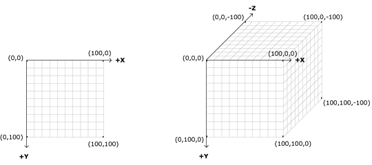
The image above illustrates the effect switching from Processing’s 2D render to Processing’s 3D render will have on the global coordinate system. You should be familiar with the image to the left from Workshop One, however, when we use ‘P3D‘ the coordinate system shifts to that of the image on the right. The z-coordinate is zero at the surface of the image, with negative z-values moving back in space.
However, when we implement PeasyCam the global coordinate system will be further altered from the image on the right to the image bellow:
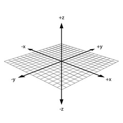
With PeasyCam the global coordinate system has now been altered to have the origin point appear at what will ‘look like‘ the centre of the canvas. The origin coordinated is still {0,0,0} however, as we are working in 3D each shift of 1 unit in either: x, y, or z will no longer be represented by a single pixel. Therefore, the size of the canvas we’ve set in the ‘size‘ function will now relate only to the size of the window and the ‘world size‘ or global coordinate system is entirely independent from the values set in the ‘size‘ function. Furthermore, as {0,0,0} appears at the centre of the canvas, we now will move both in positive values and negative values, i.e. -10 in the x will shift left, and 10 in the x will shift right from the origin and the same for y. -10 in the z will move down and 10 in the z will move up.
To illustrate this open a new Processing window, and copy the code bellow:
import peasy.*;                                  // Import the PeasyCam Library
PeasyCam cam;                                    // Declare a new variable as a PeasyCam type

void setup() {
  size(500,500, P3D);
  textMode(SHAPE);
  textSize(3);
  cam = new PeasyCam(this, 100);                 // Camera settings for 3D
  cam.setMinimumDistance(50);                    // Max camera zoom
  cam.setMaximumDistance(200);                   // Min camera zoom
}

void draw(){
  background(39, 40, 34);
   //rotateZ(0.005 * frameCount);
   strokeWeight(2);
   stroke(0,255,0);  // Green Z
     line(0, 0, 0, 0, 0, 15);
     text('Z', 0, 0, 16);
   stroke(0,0,255);  // Blue Y
     line(0, 0, 0, 0, 15, 0);
     text('Y', 0, 18, 0);
   stroke(255,0,0);  // Red X
     line(0, 0, 0, 15, 0, 0);
     text('X', 16, 0, 0);
}
Lets take a look at the code quickly as we are going to need some of the same lines of code to implement PeasyCam into our gravitational box sketch later. On line 1 we use the word ‘import‘ to tell Processing we need to include (load) a library at the beginning of our sketch, this is followed by the name of the library ‘peasy‘ and then finally followed by ‘.*‘, to indicate that Processing must load all the modules associate with the ‘peasy‘ library. Sometimes we only need a specific module in a library and then would load that module as apposed to all the modules contained in a library. Most libraries can be found through the Processing IDE ‘add more‘ button or by searching online and in most cases each library will have its own reference page providing instructions on how to import the library and some examples on how to use it. Following this we need to declare a new variable which will store the PeasyCam, much like we did early by declaring a variable which would store a singe instance of the Box class. In this case we’ve done so on line 2 by declaring a variable which is type PeasyCam and we’ve named it ‘cam‘.
In the ‘setup‘ function on line 5, we’ve told Processing to create a canvas which is 500 by 500 pixels and to use the 3D renderer ‘P3D‘. Next we need to construct an instance of a PeasyCam assigning this to our variable ‘cam‘ as done on line 8: cam = new PeasyCam(this, 100);. Then we provide ‘cam‘ with some initial settings, as shown on lines 9 and 10, which define how far-in we can zoom ‘50‘ and how far-out we can zoom ‘200‘ respectively.
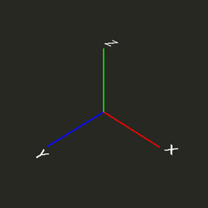
Now in ‘draw‘ we are using three lines to display a gumball widget, similar to many modelling software packages, using Processing’s ‘line‘ function, yet including a third pair of coordinates for the z-component: line(x1, y1, z1, x2, y2, z2). Each line has a unique colour and is drawn from the origin {0,0,0} to either x:15, y:15, or z:15.
When you run this sketch you will notice how the gumball widget appears at the centre of the canvas, even though we used the origin {0,0,0}, and never used a ‘translate‘ function to shift to the centre of the canvas. Each line will point in the respective direction of the three axes associated with 3D space: x, y and z.
2.2.2 Implementation: Of PeasyCam In Our Gravitational Fields Sketch
Now lets implement a PeasyCam in our gravitational box sketch, so we can better see the boxes move around in 3D space. To do so lets return to the main sketch tab and make the following changes:
import peasy.*;                               // Import the PeasyCam Library

// Objects
PeasyCam cam;                                 // Declare a new variable as a PeasyCam type
ArrayList boxes = new ArrayList();  // Declare an ArrayList of type Box

// System Parameters
int numBox = 20;                              // Declare an integer variable used to determine how many boxes we start with

void setup() {
  size(400, 400, P3D);                        // Create a canvas 400px and render in 3D (P3D)
  rectMode(CENTER);                           // Set rectMode to center
  cam = new PeasyCam(this, 1000);             // Camera settings for 3D
  cam.setMinimumDistance(100);                // Max camera zoom
  cam.setMaximumDistance(1000);               // Min camera zoom
  for (int i=0; i < numBox; i++){             // loop for as many times as set by 'numBox'
    // each loop - create a new box with randomised parameters and add it to the ArrayList
    boxes.add(new Box(random(-500,500), random(-500,500), random(-500,500), random(5, 50), random(1), randomBoolean()));
  }
}
As can be seen above we’ve included the PeasyCam library on line 1, followed by creating a new PeasyCam variable ‘cam’ on line 4. Within ‘setup‘ we’ve construct an instance of a PeasyCam assigning this to our variable ‘cam‘, though this time we’ve set a different start-zoom value of ‘1000‘ and a min-zoom of ‘100‘ and max-zoom of ‘1000‘, we may need to adjust these values later.
As mentioned earlier before we would we need to make some changes to the call to the Box constructor within our loop. This is because we can no longer use random values between 0 and ‘width’ and ‘height’ as the coordinates for a Box, as this would create boxes only in the top-left-quarter of the ‘world‘ (i.e. where x, y and z are all positive values.) We need a new range between which we can generate a random number, for this we’ve chosen ‘-500 and 500‘. Therefore a Box’s x, y and z coordinate will be a random floating point between ‘-500 and 500‘, thus, producing a random coordinate such as: {250.0, -100, -344}.
We need to make the same change for our second call to the Box constructor in the ‘mousePressed‘ function, as follows:
boxes.add(new Box(random(-500,500), random(-500,500), random(-500,500), random(5, 50), random(1), randomBoolean()));Now we can finally run the sketch and move around our world and see the boxes fly around one another in 3D space. Or not!
As you’ve probably noticed by now when you run the sketch all the boxes are on a single plane (i.e. their z-coordinate is 0). However, we’ve specified a random z coordinate between ‘-500 and 500‘ so why is this? Furthermore all our boxes are flat, would it not be better if they were cubes floating around one another? To address the first issue, we have indeed given each of our boxes a z coordinate value, however, when we draw each box we are not translating its position in 3D space, we are still simply translating it in 2D. To fix this we need to switch to the Box class tab and make some changes to our ‘draw‘ function, as follows:
  void draw() {
    posX += movX;                     // Increase the x position of the box by movX
    posY += movY;                     // Increase the y position of the box by movY
    posZ += movZ;                     // Increase the z position of the box by movZ
    pushMatrix();                     // Save global coordinate frame
      translate(posX, posY, posZ);      // Translate coordinate frame to posX, posY, posZ
      rotate(speed * frame);            // Rotate by x deg, each frame
      box(side);                        // Draw a box with the size of 'side'
    popMatrix();                      // Restore global coordinate frame
    if (spinning) {                   // If 'spinning' is true continue
      frame++;                        // Increment our frame counting variable by 1
    }
  }
Let’s take a look at the changes we’ve made and why they are necessary. Firstly, on line 4, we’ve included the line of code to add the z-component of our Box’s velocity to its z coordinate, ‘posZ‘, this is necessary otherwise a box will never move up or down in 3D space only side to side. Next we need to update our ‘translate‘ function to operate in 3D, as opposed to 2D. To do this we simply need to include a third parameter, the Box’s z coordinate or ‘posZ’. Thus each box will be correctly shifted to its correct position in both the x-axis, y-axis and z-axis. Whereas, before we effectively drew all boxes with a z coordinate of 0.
We also wanted to draw cubes rather than 2D rectangles. To achieve this we can make use of Processing’s native ‘box‘ function, which requires either a single parameter: box(size), to create a cube or three separate parameters: box(w, h, d), to create a rectangular prism. In our sketch we will simply create cubes of varying sizes. As can be seen on line 8: box(side).
Now we can run the sketch again and we should have a number of different sized cubes floating around one another in 3D space. However, the logic which controls the attraction of each box to another box is now broken, as the distance between each box is calculated incorrectly, as if all the boxes were still on a flat plane. Therefore, we need to return to the ‘attract‘ function within the Box class tab to fix this:
  void attract(Box b) {
    float d = dist(posX, posY, posZ, b.posX, b.posY, b.posZ);    // assign d the distance between this box and box b
    float diffX = b.posX - posX;                   // Assign diffX the x component difference between box b and this box
    float diffY = b.posY - posY;                   // Assign diffY the y component difference between box b and this box
    float diffZ = b.posZ - posZ;                   // Assign diffZ the z component difference between box b and this box
    movX += diffX / sq(d);                         // Increase movX by x-difference divided by the square-root of the distance
    movY += diffY / sq(d);                         // Increase movY by y-difference divided by the square-root of the distance
    movZ += diffZ / sq(d);                         // Increase movZ by z-difference divided by the square-root of the distance
}
On line 2, I’ve updated the built in Processing distance function ‘dist‘ to correctly calculate the distance between ‘this‘ box and another box ‘b‘ by including the z coordinate for each box. Now we have the correct value for the distance between two boxes in 3D space. Next we need to make two more changes. The first, line 5, is to add a new float variable ‘diffZ‘ to store the z component difference between box ‘b‘ and ‘this‘ box and lastly we need to increase the value of ‘movZ‘ by the z-difference divided by the square-root of the distance ‘d‘. Now our ‘attract‘ function works correctly for all three axes of our 3D space.
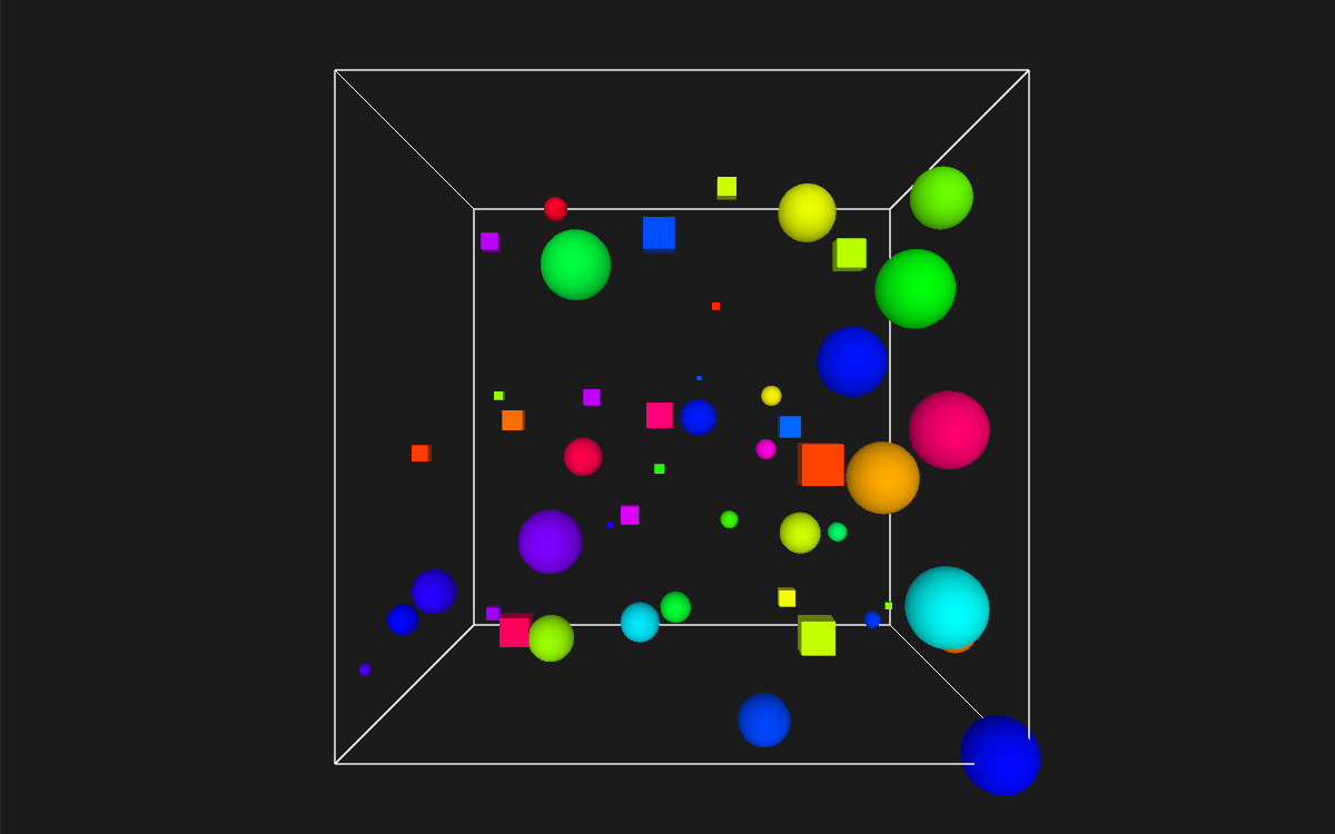
We can finally run the sketch, and we should be presented with a number of randomly sized cubes floating around one another correctly within 3D space.

Limitations: It’s important to note that when we click on the canvas we can create a new cube at a random position in space rather than at the location of the mouse, as the location of the mouse (mouseX and mouseY) does not really have any relation to a position in the 3D global coordinate frame. Furthermore, due to this fact, the code we have in ‘mousePressed‘ which enables us to click on a cube and stop or start it from spinning will no longer work and could either be removed or you could attempt to solve this problem. However, such an exercise is outside of the scope of this workshop.
2.3 Conclusion
Bellow I’ve included all the code necessary to re-create the sketch, along with some minor alterations to randomly select: the colour of each box, whether a box will be a sphere or a cube as well as alterations to the ‘attract‘ function to make it take the size of the cube or sphere into account. Thus larger objects have greater attraction than smaller objects.
/*
    * Learning Processing 3 Intermediate - Lesson 2: Three Dimensions
 *
 * Description: Basic example of implementing a class within Processing
 *
 * © Jeremy Paton (2018)
 */

import peasy.*;                               // Import the PeasyCam Library

//Objects
PeasyCam cam;                                 // Declare a new variable as a PeasyCam type
ArrayList boxes = new ArrayList();  // Declare an ArrayList of type Box

//System Parameters
int numBox = 50;                              // Declare an integer variable used to determine how many boxes we start with
int worldSize = 500;                          // Declare an integer variable used to determine size of the world

void setup() {
  fullScreen(P3D);                        // Create a canvas 400px and render in 3D (P3D)
  rectMode(CENTER);                           // Set rectMode to center
  cam = new PeasyCam(this, 2000);             // Camera settings for 3D
  cam.setMinimumDistance(100);                // Max camera zoom
  cam.setMaximumDistance(2000);               // Min camera zoom
  for (int i=0; i < numBox; i++){             // loop for as many times as set by 'numBox'
    // each loop - create a new box with randomised parameters and add it to the ArrayList
    boxes.add(new Box(random(-1*worldSize,worldSize), random(-1*worldSize,worldSize), random(-1*worldSize,worldSize), random(5, 75), random(1), randomBoolean(), random(0,255), randomBoolean()));
  }
}

void draw() {
  background(27);                // Redraw the background
  worldBox();                    // Call the worldBox function
  for (Box b: boxes) {           // Enhanced loop through ALL elements of boxes AS b
    b.draw();                    // DRAW: Call box draw function
    for (Box other: boxes) {     // Enhanced loop through ALL elements of boxes AS other
      if (b != other) {          // Check that 'this' box b is not attracting itself
        b.attract(other);        // ATTRACTOR: 'this' box b attract other box
      }
    }
  }
}

void mousePressed() {
  // Add a box at a random location to the ArrayList
  boxes.add(new Box(random(-1*worldSize,worldSize), random(-1*worldSize,worldSize), random(-1*worldSize,worldSize), random(5, 75), random(1), randomBoolean(), random(0,255), randomBoolean()));
}

// Returns a random boolean
boolean randomBoolean() {
  return random(1) < 0.5;         // If random float is larger than 0.5 return true (50% probability)
}

// Draw a wireframe box to show the world size
void worldBox(){
  pushStyle();
    noFill();
    stroke(255);
    box(worldSize*2);
  popStyle();
}
/*
* Class: a Box (literally just a box!)
*
* Description: Above ^
*
* @param {int} frame - increasing counter based on frameRate();
* @param {float} posX - x coordinate for the centre of the box
* @param {float} posY - y coordinate for the centre of the box
* @param {float} posZ - z coordinate for the centre of the box
* @param {float} side - size of the box
* @param {float} rps - revolutions per second (mapped between 0 deg and 20 deg)
* @param {boolean} spinning - on/off toggle
* @param {float} c - HSB colour value of box
* @param {boolean} t - type of box (true: box and false: sphere)
*/
class Box {
// Class Variables
int frame = 0; // Declare integer type GLOBAL variable and assign it the value 0
float posX; // Declare float type GLOBAL variable for x-position of box
float posY; // Declare float type GLOBAL variable for y-position of box
float posZ; // Declare float type GLOBAL variable for z-position of box
float movX; // Declare float type GLOBAL variable for x-component of the velocity
float movY; // Declare float type GLOBAL variable for y-component of the velocity
float movZ; // Declare float type GLOBAL variable for z-component of the velocity
float side; // Declare float type GLOBAL variable for size of box
float speed; // Declare float type GLOBAL variable for speed of box rotation
boolean spinning; // Declare boolean type GLOBAL variable and assign it true
boolean type;
float fill;
//Constructor
Box(float x, float y, float z, float s, float rps, boolean spin, float c, boolean t) {
posX = x; // Set posX equal to the parameter x
posY = y; // Set posY equal to the parameter y
posZ = z; // Set posZ equal to the parameter z
side = s; // Set side equal to the parameter s
speed = map(rps,0,1,0,0.35); // Set speed equal to (mapped between 0 deg and 20 deg)
spinning = spin; // Set spinning state equal to the parameter spin
fill = c;
type = t;
movX = random(-1,1); // Assign a random x component velocity between -1 & 1
movY = random(-1,1); // Assign a random y component velocity between -1 & 1
movZ = random(-1,1); // Assign a random y component velocity between -1 & 1
}
void attract(Box b) {
float d = dist(posX, posY, posZ, b.posX, b.posY, b.posZ); // assign d the distance between this box and box b
float diffX = b.posX - posX; // Assign diffX the x component difference between box b and this box
float diffY = b.posY - posY; // Assign diffY the y component difference between box b and this box
float diffZ = b.posZ - posZ; // Assign diffZ the z component difference between box b and this box
movX += ((diffX * (side*0.02) * (b.side*0.02)) / sq(d)); // Increase movX by x-difference divided by the square-root of the distance
movY += ((diffY * (side*0.02) * (b.side*0.02)) / sq(d)); // Increase movX by y-difference divided by the square-root of the distance
movZ += ((diffZ * (side*0.02) * (b.side*0.02)) / sq(d)); // Increase movX by z-difference divided by the square-root of the distance
}
void draw() {
posX += movX; // Increase the x position of the box by movX
posY += movY; // Increase the y position of the box by movY
posZ += movZ; // Increase the z position of the box by movZ
pushMatrix(); // Save global coordinate frame
translate(posX, posY, posZ); // Translate coordinate frame to posX, posY, posZ
rotateX(speed * frame); // Rotate by x deg, each frame
rotateY(speed * frame); // Rotate by x deg, each frame
rotateZ(speed * frame); // Rotate by x deg, each frame
pushStyle();
lights();
noStroke();
colorMode(HSB);
fill(fill, 255, 255);
if (type) {
box(side); // Draw a box with the size of 'side'
} else {
sphere(side); // Draw a sphere with the size of 'side'
}
popStyle();
popMatrix(); // Restore global coordinate frame
if (spinning) { // If 'spinning' is true continue
frame++; // Increment our frame counting variable by 1
}
}
}3. Vectors: Motion And Acceleration
Lesson three can be considered a more self-contained lesson, in comparison to the first two lessons of this workshop, in which we are going to explore the programming of motion in more detail. Lesson three will introduce the most basic building block for programming motion — the vector. Whilst we’ve touched on calculating motion, such as in the ‘attract‘ function, in the previous lesson, this lesson will introduce a more efficient way to store location and direction by using vectors, something we did not use in our ‘attract‘ function. We will also introduced other types of motion such as, separation as well as calculating acceleration for an objects motion.
This lesson will provide a foundation to move onto lesson four in which we will use vectors to apply forces, such as gravity or wind to an object.
Key programming concepts:
Vectors (PVector) and Vector Maths
3.1 Introduction
‘PVectors‘ as they are referred to within Processing, are a class used to describe a two or three dimensional vector. What exactly is a vector? There are in fact multiple varying definitions for the term vector each pertaining to different fields of study. However, the definition of a vector we are look for would be an Euclidean vector (named for the Greek mathematician Euclid and also known as a geometric vector). A vector can be though of, or visualised, as as an arrow; the direction is indicated by where the arrow is pointing, and the magnitude by the length of the arrow itself:

The above illustration shows a vector which is drawn as an arrow from point A to point B and serves as an instruction for how to travel from A to B. In other words, in the diagram a vector (drawn as an arrow) has magnitude (length of arrow) and direction (which way it is pointing).
The ‘PVector‘ datatype, stores two or three variables. First the components of the vector (x,y for 2D, and x,y,z for 3D), second the magnitude or velocity and/or third the acceleration. We can obtain the components of a vector using dot notation to get the: ‘vector.x, vector.y, vector.z‘, we can also obtain the magnitude and heading through dot notation calling ‘magnitude()‘ and/or ‘heading()‘ respectively. Technically, position is a point {x,y,z} whilst velocity and acceleration are vectors, but this is often simplified to consider all three as vectors.
As an example lets consider a rectangle moving across the canvas, at any given moment it has a position (the object’s location, expressed as a point), a velocity (the rate at which the object’s position changes per time unit, expressed as a vector), and acceleration (the rate at which the object’s velocity changes per time unit, expressed as a vector).
3.2 Using PVectors
Before jumping into more detail about vectors, let’s look at a basic Processing example that demonstrates why we should care about vectors in the first place. To do this we will write a basic bouncing ball sketch, first without using vectors:
float x = 100;          // X location of ball
float y = 100;          // Y location of ball
float xSpeed = 1;       // X speed of ball
float ySpeed = 3.3;     // Y speed of ball

void setup() {
  size(900,200);
}

void draw() {
  background(39, 40, 34);
  noStroke();
  fill(255);

  x += xSpeed;                   // Every frame move the ball based on its xSpeed
  y += ySpeed;                   // Every frame move the ball based on its xSpeed

  if ((x > width) || (x < 0)) {  // Check for bounce
    xSpeed = xSpeed * -1;        // Inverse the xSpeed
  }
  if ((y > height) || (y < 0)) {
    ySpeed = ySpeed * -1;        // Inverse the ySpeed
  }

  ellipse(x,y,25,25);            // Draw ball
}In the above sketch, we have a very simple world — a blank canvas with a circular shape (a ball) travelling around. This ball has some properties, which are represented in the code as variables which define the balls location: ‘x‘ and ‘y‘, and the balls speed: ‘xSpeed‘ and ‘ySpeed‘. In a more advanced sketch we could include even more properties, such as:
- Acceleration — xAcceleration and yAcceleration
- Target — xTarget and yTarget location
- Wind — xWind and yWind
- Friction — xFriction and yFriction
As we can see for each new property we want to add to this world we need to add two new variables and this is only a 2D world. In a 3D world, we’ll need three variables for each property: ‘x, y, z‘, ‘xSpeed, ySpeed, zSpeed‘, and so on. Wouldn’t it be nice if we could simplify our code and use fewer variables? Well this is in fact possible with vectors, by replacing our properties as follows:
PVector pos;            // Location of ball stored as a vector
PVector speed;          // Speed of ball stored as a vector
This is the first step towards using vectors, however this won’t provide anything new yet. Simply adding vectors does not magically make our Processing sketches simulate physics. However, they will drastically simplify your code and provide a set of functions for common mathematical operations which occur regularly while programming motion.
For now our introduction to vectors will live in two dimensions, as it’s not entirely necessary to over complicate things with a third dimension just yet, and as shown in the previous section: 2.2.2 Implementation: Of PeasyCam In Our Gravitational Fields Sketch converting a sketch from 2D to 3D is not as daunting a task as one you may have thought it to be. All of these examples can be fairly easily extended to three dimensions (and the class we will use — PVector — naively allows for three dimensions.)
We’ve actually already, unintentionally, explained what a vector is in the previous section: 1.7 Gravitational Fields, we can think of of a vector as the difference between two points. Consider how you might go about providing instructions to walk from one point to another:


(-3, 4)                 Walk three steps west; turn and walk four steps north.
(3, -2)                 Walk three steps east; turn and walk 2 steps south.
We have already done this before whilst programming motion. For every frame of animation (i.e. a single cycle through Processing’s draw() loop), you instruct each object on the screen to move a certain number of pixels horizontally and a certain number of pixels vertically. This could be expressed at for every frame: ‘new location = velocity applied to current location‘. This is essentially what we were doing back in our ‘attract‘ function.
If velocity is a vector (the difference between two points), what is location? Is it a vector too? Technically, one might argue that location is not a vector, since it’s not describing how to move from one point to another — it’s simply describing a singular point in space. Nevertheless, another way to describe a location is the path taken from the origin to reach that location. Hence, a location can be the vector representing the difference between location {x,y,z} and origin {0,0,0}.
Let’s briefly examine the underlying data for both location and velocity. In the bouncing ball example in which we have the following two PVectors: ‘location’ and ‘speed‘. Notice how we are storing the same data for both — two floating point numbers, an x and a y. If we were to write a vector class ourselves, say if we were using a langue that did not have a vector class, we’d begin with something rather basic, like so:
class PVector {

  float x;
  float y;
  // PVector constructor
  PVector(float x_, float y_) {
    x = x_;
    y = y_;
  }
}
Fortunately Processing has a vector class, PVector, so we don’t need to do this. Though at its core, a PVector is just a convenient way to store two values (or three, as we’ll see in 3D examples). Thus for us to start converting our bouncing ball example to use a PVector we would replace our initial property variables, ‘x‘, ‘y‘, ‘xSpeed‘ and ‘ySpeed‘, with the following:
PVector location = new PVector(100,100);      // Location of ball stored as a vector
PVector velocity = new PVector(1,3.3);        // Speed of ball stored as a vector
Let’s take a look at the above code. First we declare two new PVector type variables ‘location‘ and ‘velocity‘ followed by immediately assigning them with a new PVector. Notice the use of the word ‘new‘ as we have previously done when creating a new Box in the previous lessons, this is always used when we assign a class-type variable a new instance of a class, such as a color, PVector, or our Box. We follow this by the parameter(s) of the PVector: PVector(x, y, z). Now that we have two vector objects, ‘location‘ and ‘velocity‘, we’re ready to implement the algorithm for motion: location = location + velocity.
Previously within ‘draw‘ we incremented ‘x‘ by ‘xSpeed‘ and ‘y‘ by ‘ySpeed‘ to apply motion (a change in position for each frame), in an ideal world, we would be able to rewrite the above, using PVectors, as: location = location + velocity;
However, in Processing, the addition operator ‘+‘ is reserved for primitive values (integers, floats, etc.) only. Processing doesn’t know how to add two PVector objects together any more than it knows how to add two PFont objects or Box objects. This is since vectors represent groupings of values, therefore, we cannot simply use traditional addition/multiplication/etc. Instead we need to do some ‘vector’ maths. Fortunately for us, the PVector class includes functions for common mathematical operations.
3.2.1 Vector Maths: Addition
Before we take a look at the PVector class and its ‘add()‘ method, let’s take a look at how addition is implemented in the PVector class itself by writing our own ‘add‘ function which takes another PVector object as its argument. We would write the following (this is purely for the sake of learning since it’s already implemented for us in Processing):
class PVector {

  float x;
  float y;
  // PVector constructor
  PVector(float x_, float y_) {
    x = x_;
    y = y_;
  }

  void add(PVector v) { // Add another PVector to this PVector
    y = y + v.y;        // Add the x components together
    x = x + v.x;        // Add the y components together
  }
}
Now that we see how the ‘add‘ function essentially works inside of the PVector class, we can return to our bouncing ball example which requires the correct vector addition implementation of our location + velocity algorithm, to do this we change the following line to:
  // location = location + velocity;   // Incorrect method
  location.add(velocity);              // Vector addition
All that remains are a few more changes to the syntax of our code to correctly make reference to the bouncing ball’s location vector x and y components. To complete the sketch we would write the following:
PVector location;        // Declare new vector variable for ball location
PVector velocity;        // Declare new vector variable for ball speed

void setup() {
  size(900,200);
  location = new PVector(100,100);      // Assign location a new vector x and y value
  velocity = new PVector(1,3.3);        // Assign velocity a new vector x and y value
}

void draw() {
  background(39, 40, 34);
  noStroke();
  fill(255);

  location.add(velocity);                          // Vector addition

  if ((location.x > width) || (location.x < 0)) {  // Check for bounce
    velocity.x = velocity.x * -1;                  // Inverse the velocity
  }
  if ((location.y > height) || (location.y < 0)) {
    velocity.y = velocity.y * -1;                  // Inverse the velocity
  }

  ellipse(location.x,location.y,25,25);            // Draw ball
}
We’ve made a couple of simple changes to the code. First we’ve updated the edge detection if statements, on lines 17 and 20, to get the ball’s x and y coordinates from the ball’s ‘location‘ vector, using dot notation: location.x and location.y. We’ve done the same on line 24, when drawing the ellipse. Lastly, we need to invert the x and y components of the ‘velocity‘ vector which we’ve done on lines 18 and 21, again using dot notation.
Now, you may be somewhat disappointed. After all, this may initially appear to have made the code more complicated than the original version. While this is a reasonable critique, it’s important to understand that we haven’t fully realised the potential of programming with vectors just yet. Looking at a simple bouncing ball and only implementing vector addition is just the first step. As we proceed into more complex worlds containing multiple objects and multiple forces (next lesson), the benefits of PVector will become more apparent.
3.2.2 More Vector Maths
Addition is only the first step, in learning about vector maths. There are many mathematical operations that are commonly used with vectors. Below is a comprehensive list of the operations available as functions within the PVector class. We’ll go through a few of the key ones now.
- add() — add vectors
- sub() — subtract vectors
- mult() — scale the vector with multiplication
- div() — scale the vector with division
- mag() — calculate the magnitude of a vector
- setMag() – set the magnitude of a vector
- normalize() — normalize the vector to a unit length of 1
- limit() — limit the magnitude of a vector
- heading() — the 2D heading of a vector expressed as an angle
- rotate() — rotate a 2D vector by an angle
- lerp() — linear interpolate to another vector
- dist() — the Euclidean distance between two vectors (considered as points)
- angleBetween() — find the angle between two vectors
- dot() — the dot product of two vectors
- cross() — the cross product of two vectors (only relevant in three dimensions)
- random2D() – make a random 2D vector
- random3D() – make a random 3D vector
3.2.3 Vector Maths: Subtraction
Now that we’ve covered addition, let’s quickly explore subtraction. This one’s not so bad, simply replace the plus sign with a minus! Thus the ‘subtract‘ function inside the PVector class would look similar to this:
  void sub(PVector v) { // Subtract another PVector from this PVector
    y = y - v.y;        // Subtract the x components
    x = x - v.x;        // Subtract the y components
  }
The following example demonstrates vector subtraction by calculating the difference between two points, in this case the mouse location and the centre of the canvas:
PVector centre;            // Declare new vector variable for centre location
PVector mouse;             // Declare new vector variable for mouse location

void setup() {
  size(900,200);
  centre = new PVector(width/2,height/2);    // Assign the centre vector the centre of the canvas
}

void draw() {
  stroke(255);
  background(39, 40, 34);
  mouse  = new PVector(mouseX,mouseY);       // Each frame update mouse vector with the location of the mouse
  mouse.sub(centre);                         // Calculate the difference between mouse location and centre location
  translate(centre.x,centre.y);              // Translate the centre location (canvas centre)
  line(0,0,mouse.x,mouse.y);                 // Draw a line from canvas origin to mouse vector location
}Again the above code is a rather unnecessary complication to the task of drawing a line from the canvas centre to the mouse location, however, it’s still a reasonably good way to visually represent how vector subtraction operates.
3.2.4 Vector Maths: Multiplication
Multiplication on the other hand operates a little differently. When we talk about multiplying a vector, what we typically mean is scaling a vector. If we wanted to scale a vector to twice its size or one-third of its size (leaving its direction the same), we would say: ‘multiply the vector by 2‘ or ‘multiply the vector by 1/3.‘ Note that we are multiplying a vector by a scalar, a single number, not another vector.
Therefore, the function inside the PVector class would be written as follows:
  void mult(float n) { // Multiply the components of a vector
   x = x * n;          // X component is multiplied by a number
   y = y * n;          // Y component is multiplied by same number
 }
To implement vector multiplication in code we can write the following:
PVector center;            // Declare new vector variable for center location
PVector mouse;             // Declare new vector variable for mouse location

void setup() {
  size(900,200);
  center = new PVector(width/2,height/2);    // Assign the center vector the center of the canvas
}

void draw() {
  stroke(255);
  background(39, 40, 34);
  mouse  = new PVector(mouseX,mouseY);       // Each frame update mouse vector with the location of the mouse
  mouse.sub(center);                         // Calculate the difference between mouse location and center location
  mouse.mult(0.5);                           // Reduce (scale) the vector by 50% of the distance between the mouse and center
  translate(center.x,center.y);              // Translate the center location (canvas centre)
  line(0,0,mouse.x,mouse.y);                 // Draw a line from canvas origin to mouse vector location
}We’ve already stated that by multiplying a vector we are in fact scaling the vector. In the above example our vector is the visible line pointing from the canvas centre to the mouse location, which is first calculated as the difference between the these two points. We’ve included vector multiplication on line 14: mouse.mult(0.5);, here we are telling Processing to scale the ‘mouse‘ vector by the scalar value ‘0.5’. In other words, scale the size (length) of the mouse vector by 50% of its original length. Try moving the mouse further away from the canvas centre and notice how the line is only ever half the length of the total distance between the canvas centre and the mouse location.
3.2.4 Vector Magnitude
Vector Multiplication and division, are means by which the length of the vector can be changed without affecting direction. Perhaps you’re thinking: “Ok, so how do I know what the length of a vector is? I know the x and y components, but how long is the actual arrow?” The length of a vector is also referred to as the magnitude and being able to calculate the length of a vector is incredibly useful and important.

Notice, in the diagram on the left, how the vector, drawn as an arrow and two components (x and y), creates a right triangle. The sides are the components and the hypotenuse is the arrow itself. We’re lucky to have this right triangle because, a Greek mathematician named Pythagoras developed a useful formula to describe the relationship between the sides and hypotenuse of a right triangle. The Pythagorean theorem is ‘a‘ squared plus ‘b‘ squared equals ‘c‘ squared. Or in the case of the triangle on our left: ‘x‘ squared plus ‘y‘ squared equals ‘v‘ squared.
With this formula, it’s possible to compute the magnitude ‘mag‘ of the vector ‘v‘, within the the PVector class as follows:
  float mag() {              // Calculate the length 'mag' of this vector
    return sqrt(x*x + y*y);  // Implement Pythagorean theorem to solve the length
  }
To illustrate this let’s draw a rectangle with its width equal to the hypotenuse or magnitude of the vector created between the centre of the canvas and the mouse position, or the ‘mouse‘ vector. To do so we will call the ‘mag()‘ function which returns a floating point value, which is the length of the vector and use this value as the rectangle’s width:
PVector centre;            // Declare new vector variable for centre location
PVector mouse;             // Declare new vector variable for mouse location

void setup() {
  size(900,200);
  centre = new PVector(width/2,height/2);    // Assign the centre vector the centre of the canvas
}

void draw() {
  noStroke();
  background(39, 40, 34);
  mouse  = new PVector(mouseX,mouseY);       // Each frame update mouse vector with the location of the mouse
  mouse.sub(centre);                         // Calculate the difference between mouse location and centre location

  float hypotenuse = mouse.mag();
  fill(255,0,255);
  rect(0,0,hypotenuse,10);

  stroke(255);
  translate(centre.x,centre.y);              // Translate the centre location (canvas centre)
  line(0,0,mouse.x,mouse.y);                 // Draw a line from canvas origin to mouse vector location
}3.2.4 Normalizing Vectors
The magnitude function opens the door to many possibilities, the first of which is normalization. Normalizing refers to the process of making something “standard” or, well, “normal.” In the case of vectors, let’s assume for the moment that a standard vector has a length of 1. This is the way Processing is set to implement normalize and will always set the length of the vector to 1 unit. To normalize a vector, therefore, is to take an existing vector of any length and, without changing its position, set its length to 1, turning it into what is called a unit vector. A unit vector is rather useful as it describes a vector’s direction without regard for its length, having a unit vector readily accessible will prove useful as we start to implement forces in the next lesson. Within the PVector class the ‘normalize’ function would be written as so:
  void normalize() {      // Set vectors magnitude to 0
    float m = mag();
    if (m != 0) {         // Make sure we don't divide by 0 if mag is 0
      div(m);             // divide the magnitude by itself (i.e. 5/5 = 1)
    }
  }
Once again to illustrate this let’s implement the ‘normalize’ function into our previous sketch. Doing so will set the length of the ‘mouse‘ vector to 1 unit, and as we move the mouse cursor around the vector will point in that direction but will not change length or magnitude. We can implement this as follows:
PVector centre;            // Declare new vector variable for centre location
PVector mouse;             // Declare new vector variable for mouse location

void setup() {
  size(900,200);
  centre = new PVector(width/2,height/2);    // Assign the centre vector the centre of the canvas
}

void draw() {
  noStroke();
  background(39, 40, 34);
  mouse  = new PVector(mouseX,mouseY);       // Each frame update mouse vector with the location of the mouse
  mouse.sub(centre);                         // Calculate the difference between mouse location and centre location

  mouse.normalize();                         // Set the mouse vectors magnitude to 1 unit
  mouse.mult(50);                            // 1 unit is hard to see, so lets scale the vector up

  stroke(255);
  translate(centre.x,centre.y);              // Translate the centre location (canvas centre)
  line(0,0,mouse.x,mouse.y);                 // Draw a line from canvas origin to mouse vector location
}Once we have ‘normalized‘ the mouse vector, as seen on line 15: mouse.normalize();, the length of the line drawn on the screen will always be 1 pixel. If you run the sketch you may vaguely see the line move to point in the direction of the mouse cursor, however, 1 pixel is a little small to see this, thus we can scale up the vector by 50 times. To do so we will use the PVector ‘mult‘ function to multiple the vector by 50, as see on line 16: mouse.mult(50);. Now when we run the sketch the line is easier to see.
3.3 Vector Motion 101: Velocity
All this vector maths stuff sounds useful and is probably something we should know about, but why? How will it actually help us write code? In all honesty we need to be a little patience. It will take some time before the awesomeness of using the PVector class fully comes to light. This is a pretty common occurrence when first learning a new data structure. For example, when you first learn about an array and ArrayList, it might seem like much more work to use an array than to just have several variables stand for multiple things. But that plan quickly breaks down when you need a hundred, or a thousand, or ten thousand things. The same can be true for PVector. What might seem like more work now will pay off later, and pay off quite nicely. And you don’t have to wait too long, as your reward will come in the next lesson.
But first there are two final, and very important points we need to cover and those are velocity and acceleration. What does it mean to program motion using vectors? As demonstrated at the beginning of this lesson: 3.2 Using PVectors — the bouncing ball. An object on the canvas has a location (where it is at any given moment) as well as a velocity (instructions for how it should move from one frame to the next). Velocity is added to location, for each frame:
location.add(velocity);Followed by drawing the object at that new location:
ellipse(location.x,location.y,25,25);This is what we refer to as Motion 101:
- Add velocity to location
- Draw object at location
In our bouncing ball sketch, we have included all of this code within Processing’s main tab, within ‘setup‘ and ‘draw‘ functions. What we want to do now is move towards encapsulating all of the logic for motion inside of a class, much like we’ve already done at the end of Workshop 1. This way, we can create a foundation for programming moving objects in Processing. Beyond this point the lesson assumes you have experience with objects and classes in Processing, from the previous workshop!
In this case, we’re going to create a generic Vehicle class, which will describe a thing moving around the screen. This is the first stage in our long-term goal towards an autonomous agent. Thus we must consider the following two questions:
- What data does a Vehicle require?
- What functionality does a Vehicle have?
Our Motion 101 algorithm provides us the answers to these questions. A Vehicle object has two primary pieces of data: location and velocity, which are both PVector objects. So to begin lets create a new Vehicle class in a new tab (name the tab Vehicle) and the class ‘Vehicle‘, as so:
class Vehicle {

  PVector location;
  PVector velocity;
The Vehicle’s functionality is just as simple. The Vehicle needs to move and it needs to be seen. Therefore, we will implement these capabilities as functions named ‘update()‘ and ‘display()‘. We’ll put all of our motion logic code in ‘update()‘ and draw the object in ‘display()‘, as follows:
  void update() {
    location.add(velocity);          // Euclidean vector movement
  }

  void display() {                   // The vehicle is displayed
    pushStyle();
      noStroke();
      fill(175);
      ellipse(location.x, location.y, 20, 20);
    popStyle();
  }
So far what we’ve written should seem somewhat familiar as it builds upon everything we’ve learnt thus far. Therefore, you should have picked up on the fact that we’ve forgotten one crucial function: the object’s constructor. The constructor always has the same name as the class and is where we give instructions on how to set up the object. It’s called by invoking the new operator, in the main sketch tab, which we will do as follows, a little later:
Vehicle v = new Vehicle();For now let’s arbitrarily decide to initialize our Vehicle object by giving it a random location and a random velocity, as follows:
  Vehicle() {
    location = new PVector(random(width),random(height));
    velocity = new PVector(random(-2,2),random(-2,2));
    }
Let’s finish off the Vehicle class by developing a function to determine what the object should do when it reaches the edge of the canvas. For now let’s do something simple, and just have it wrap around the edges:
  void checkEdges() {                // When it reaches one edge, set location to the other

    if (location.x > width) {        // Check for width
      location.x = 0;
    } else if (location.x < 0) {
      location.x = width;
    }

    if (location.y > height) {       // Check for height
      location.y = 0;
    } else if (location.y < 0) {
      location.y = height;
    }
  }
For now the Vehicle class is finished, so we need to look at what needs to be done in our main program. We first declare a Vehicle object:
Vehicle vehicle;Then initialize the vehicle within ‘setup()‘:
vehicle = new vehicle();and call the appropriate vehicle functions within ‘draw()‘:
vehicle.update();
vehicle.checkEdges();
vehicle.display();
Bellow is an example for reference:
Vehicle vehicle;

void setup(){
  size(900,200);
  vehicle = new Vehicle();
}

void draw(){
  background(39, 40, 34);
  vehicle.update();
  vehicle.checkEdges();
  vehicle.display();
}
class Vehicle {
PVector location;
PVector velocity;
Vehicle() {
location = new PVector(random(width), random(height));
velocity = new PVector(random(-3, 3), random(-3, 3));
}
void update() {
location.add(velocity); // Euclidean vector movement
}
void checkEdges() { // When it reaches one edge, set location to the other
if (location.x > width) { // Check for width
location.x = 0;
} else if (location.x < 0) {
location.x = width;
}
if (location.y > height) { // Check for height
location.y = 0;
} else if (location.y < 0) {
location.y = height;
}
}
void display() { // The vehicle is displayed
pushStyle();
noStroke();
fill(255, 0, 255);
ellipse(location.x, location.y, 50, 50);
popStyle();
}
}3.4 Vector Motion 101: Acceleration
Congratulation, you’ve created a vehicle class implementing PVector. Therefore, currently, you should feel comfortable with two things:
- What a PVector is
- How we can use PVectors inside of an object (class) to keep track of its location and movement.
This is an excellent first step. Before standing ovations and screaming fans, however, we need to make one more, somewhat bigger step forward. After all, watching the Motion 101 example above is fairly boring — the circle never speeds up, never slows down, and never turns. For more interesting motion, for motion similar to that which appears in the real world around us, we need to add one more PVector to our class — acceleration.
The strict definition of acceleration we’re using here is: the rate of change of velocity. Let’s think about that definition for a moment. Is this a new concept? Not really. Velocity is defined as the rate of change of location. In essence, we are developing a “trickle-down” effect. Acceleration affects velocity, which in turn affects location. In code, this reads:
velocity.add(acceleration);
location.add(velocity);
The above code should not seem too abstract at this point as we are essentially using the PVector ‘add‘ function twice, one after the other. Firstly to update the velocity at which the object is moving by adding the acceleration (or deceleration, ‘–‘ value) to the velocity followed by adding the newly calculated velocity to the objects present location.
As a challenge, from this point forward, let’s make a rule for ourselves. Let’s write every example in the rest of this lesson without ever touching the value of velocity and location (except to initialize them). In other words, our goal now for programming motion is: Come up with an algorithm for how we calculate acceleration and let the trickle-down effect work its magic. (In truth, you’ll find reasons to break this rule, but it’s important to illustrate the principles behind our motion algorithm.) And so we need to come up with some ways to calculate acceleration:
3.4.1 Types of Acceleration Algorithms?
- A constant acceleration
- A totally random acceleration
- Acceleration towards the mouse
The above is not an exhaustive list and we unfortunately don’t have time to demonstrate all these examples in this workshop, for now we will focus on; constant acceleration and Acceleration towards the mouse.
In order to demonstrate Algorithm 1: a constant acceleration, we will need to make some changes to our Vehicle class. Whilst this type of acceleration is not particularly interesting, it is the simplest and will help us begin incorporating acceleration into our code. The first thing we need to do is add another PVector to the Vehicle class:
class Vehicle {

  PVector location;                  // PVector for vehicle's location
  PVector velocity;                  // PVector for vehicle's velocity
  PVector acceleration;              // NEW: PVector for vehicle's acceleration
This is not enough obviously to implement acceleration into our vehicle, we now need to incorporate acceleration into the Vehicle’s ‘update()‘ function:
  void update() {                    // Euclidean vector movement
    velocity.add(acceleration);      // NEW: Calculate the change of velocity
    location.add(velocity);          // Calculate the change of position
  }
We’re almost done. The only missing piece is the initialization in the constructor: ‘Vehicle()‘. Here let’s rather start the Vehicle object in the middle of the canvas and with an initial velocity of zero:
  Vehicle() {
    location = new PVector(width/2,height/2);
    velocity = new PVector(0,0);
  }
When we run the sketch this will result in the the object being at rest. We don’t have to worry about velocity anymore, as we are controlling the Vehicle’s motion entirely with acceleration. Speaking of which, according to Algorithm 1: a constant acceleration, our first sketch involves constant acceleration. So let’s select a value:
  Vehicle() {
    location = new PVector(width/2,height/2);
    velocity = new PVector(0,0);
    acceleration = new PVector(-0.001,0.01);
  }
Maybe you’re thinking, “Hmm… those values seem awfully small!” That’s correct, they are quite small indeed. It’s important to realise that our acceleration values (measured in pixels whilst in 2D) accumulate over time in velocity, about thirty times per second depending on our sketch’s frame rate. And so to keep the magnitude of the velocity vector within a reasonable range, our acceleration values should remain quite small. We can also help this cause by incorporating the PVector function ‘limit()‘, as follows:
velocity.limit(10); // NEW: Limit the top speedLimit will do the following: What is the magnitude of velocity? If it’s less than 10, just leave it as is. However, if it’s more than 10, however, reduce it to 10!
Let’s take a look at the changes to the Mover class, complete with ‘acceleration’ and ‘limit()‘.
Vehicle vehicle;

void setup(){
  size(900,200);
  vehicle = new Vehicle();
}

void draw(){
  background(39, 40, 34);
  vehicle.update();
  vehicle.checkEdges();
  vehicle.display();
}
class Vehicle {
PVector location; // PVector for vehicle's location
PVector velocity; // PVector for vehicle's velocity
PVector acceleration; // NEW: PVector for vehicle's acceleration
Vehicle() {
location = new PVector(width/2,height/2);
velocity = new PVector(0,0);
acceleration = new PVector(-0.001,0.01);
}
void update() { // Euclidean vector movement
velocity.add(acceleration); // NEW: Calculate the change of velocity
velocity.limit(10); // NEW: Limit the top speed
location.add(velocity); // Calculate the change of position
}
void checkEdges() { // When it reaches one edge, set location to the other
if (location.x > width) { // Check for width
location.x = 0;
} else if (location.x < 0) {
location.x = width;
}
if (location.y > height) { // Check for height
location.y = 0;
} else if (location.y < 0) {
location.y = height;
}
}
void display() { // The vehicle is displayed
pushStyle();
noStroke();
fill(255, 0, 255);
ellipse(location.x, location.y, 50, 50);
popStyle();
}
}3.5 Interactivity with Acceleration
We will finish this lesson by attempting something a bit more complex and a great deal more useful. We’ll dynamically calculate an object’s acceleration according to a rule stated in Algorithm 3 the object accelerates towards the mouse.
Anytime we want to calculate a vector based on a rule or a formula, we need to compute two things: magnitude and direction. Let’s start with direction. We know the acceleration vector should point from the object’s location towards the mouse location. Let’s say the object is located at the point {x,y} and the mouse at {mouseX,mouseY}. The acceleration is directly proportional to the distance or magnitude of the vector created between the mouse cursor and the object, the further away the faster the object will travel towards the mouse and the closer it gets the slower it will travel.
This will be similar to how we created a vector pointing from the centre of the canvas to the mouse location, only now we are pointing from the objects location to the location of the mouse. To do this we used the PVector ‘sub‘ (subtract) function to find the difference between to PVectors. Let’s write the above using PVector syntax. Assuming we are in the Vehicle class and thus have access to the vehicles’s PVector location, we then have:
    PVector target = new PVector(mouseX,mouseY);
    /* We use the static reference to sub() as we want a NEW PVector
       pointing from the target to another the vehicle's location.
    */
    PVector dir = PVector.sub(target,location);
We now have a new PVector, called ‘dir‘, which points from the vehicles’s location all the way to the mouse, ‘target‘. If the object were to actually accelerate using that vector, it would appear instantaneously at the mouse location. This does not make for good animation, of course, and what we want to do now is decide how quickly that object should accelerate toward the mouse.
In order to set the magnitude (whatever it may be) of our ‘acceleration’ PVector, we must first Normalize that direction ‘dir‘ vector. If we can shrink the vector down to its unit vector (of length one) then we have a vector that tells us the direction and can easily be scaled to any value. One multiplied by anything equals anything.
float anything = ?????
dir.normalize();
dir.mult(anything);
In summary, we’ve taken the following steps:
- Calculate a vector that points from the object to the target location: ‘dir‘
- Normalize that vector (reducing its length to 1)
- Scale that vector to an appropriate value (by multiplying it by some value)
- Assign that vector to acceleration
And here are those steps in the ‘update()‘ function itself:
Vehicle vehicle;

void setup(){
  size(900,200);
  vehicle = new Vehicle();
}

void draw(){
  background(39, 40, 34);
  vehicle.update();
  vehicle.display();
}
class Vehicle {
PVector location; // PVector for vehicle's location
PVector velocity; // PVector for vehicle's velocity
PVector acceleration; // PVector for vehicle's acceleration
float topSpeed; // NEW: Vehicle's top speed
Vehicle() {
location = new PVector(width/2,height/2); // Vehicle starts at centre of canvas
velocity = new PVector(0,0); // Vehicle starts at rest
topSpeed = 8; // NEW: set top speed to 8
}
void update() { // Euclidean vector movement
PVector target = new PVector(mouseX,mouseY);
/* We use the static reference to sub() as we want a NEW PVector
pointing from the target to another the vehicle's location.
*/
PVector dir = PVector.sub(target,location);
dir.normalize(); // Set dir magnitude to 1
dir.mult(0.5); // Scale magnitude by 50%
acceleration = dir; // Assign acceleration to dir
velocity.add(acceleration); // Calculate the change of velocity
velocity.limit(topSpeed); // Limit the top speed to 'topSpeed'
location.add(velocity); // Calculate the change of position
}
void display() { // The vehicle is displayed
pushStyle();
noStroke();
fill(255, 0, 255);
ellipse(location.x, location.y, 50, 50);
popStyle();
}
}You may be wondering why the circle doesn’t come to rest when it reaches the target. It’s important to note that the object moving has no knowledge about trying to stop at a destination; it only knows where the destination is and tries to go there as quickly as possible. Going as quickly as possible means it will inevitably overshoot the location and have to turn around, again going as quickly as possible towards the destination, overshooting it again, and so on and so forth.
This example is remarkably close to the concept of a gravitational attraction field (which we explored earlier however, without the use of vectors). However, one thing is missing here which is the strength of gravity (magnitude of acceleration) is inversely proportional to distance. This means that the closer the object is to the mouse, the faster it accelerates.
We’ve come to the end of lesson three, and whilst it may feel like we’ve covered everything there is to know about PVectors we have in fact only touched the surface. If you’re interested in exploring vector motion in more detail I would strongly encourage you to take a look at the book: The Nature of Code by Daniel Shiffman, which was incredibly useful in helping producing this lesson and covers the topic of vector motion in greater detail.
As an exercise to do yourself try implementing the above example with a variable magnitude of acceleration, stronger when it is either closer or farther away or maybe try using an array to have multiple vehicles visible on the canvas.
4. Autonomous Agents
Lesson four will extend what we’ve learnt about in lesson three: vectors, by adapting our Vehicle class into what is referred to as an agent or Agent class. This lesson aims to introduce you to the concept of an autonomous agent and provide a brief and basic example of how to implement multiple agents to create swarm like behaviours. Due to time availability, or the lack there of, of our all day workshops we’ve had to very quickly get to grips with vectors and vector motion. We have in fact jumped-the-gun, so to speak, by moving onto autonomous agents and completely skipped over other types of vector motion such as; forces, oscillation and more complex multi-vehicle driven systems such as, particle system. All of these are highly valuable fields to learn about and will assist in your understanding of both vector motion as well as programming complex multi-vehicle driven systems including autonomous agents, which we are about to look at.
Therefore, I would highly recommend that you read the book: The Nature of Code by Daniel Shiffman, where all these topic are discussed in considerably more detail!
However, let us consider what we’ve been designing so far? Inanimate objects. Lifeless shapes sitting on our screens that flop around when affected by external forces. What if we could breathe life into those shapes? What if those shapes could live by their own rules? This is what we will tackle in this lesson — the development of autonomous agents.
Key programming concepts:
Agents, agency, functional cylce and PVectors
3.1 Introduction
Alright! That’s all good and well, but what is an agent? The term autonomous agent usually refers to an entity that makes its own choices about how to act in its environment without any influence from a leader or global plan. For us, “acting” will mean moving. This addition is a significant conceptual leap as we are now expecting our box or shape or vehicle to have “desire” to move itself somewhere or interact with something off its own accord. The cause for change or the force for change occurs internally. There are three key characteristics of an agent:
- An Agent is situated: it is in continuous interaction with its environment, perceiving its environment through sensors and acting upon that environment using effectors.
- An Agent is a (computational) system. Since an agent is in interaction with an environment, that environment can, and in most situations will, demand action upon the agent – potentially within a certain amount of time. (So when designing an agent-based system, we (may) have to take into account that an agent’s resources are limited. i.e. it can die.)
- An Agent is intentional: an agent is best described from an intentional stance. Systems which are less complex, are better described from a mechanical stance and are not agents by our definition: i.e., a light switch, steam governor or thermostat.
The good news is, while the concept of forces that come from within is a major shift in our design thinking, our code base will barely change, as these desires and actions are simply that — forces.
In the late 1980s, computer scientist Craig Reynolds developed algorithmic steering behaviours for animated characters. These behaviours allowed individual elements to navigate their digital environments in a “lifelike” manner with strategies for fleeing, wandering, arriving, pursuing, evading, etc. Used in the case of a single autonomous agent, these behaviours are fairly simple to understand and implement. In addition, by building a system of multiple characters that steer themselves according to simple, locally based rules, surprising levels of complexity emerge. The most famous example is Reynolds’s “boids” model for “flocking/swarming” behaviour. — Daniel Shiffman
3.2 Vehicles and Steering
Now that we have a rudimentary understanding of the core concepts behind autonomous agents, we can begin writing the code. There are many places where we could start such as, artificial simulations of ant and termite colonies which make for great demonstrations of systems of autonomous agents. However, for now we will begin by examining agent behaviours that build on the work we’ve done in previous lessons this workshop: modelling motion with vectors and driving motion with forces. I actually foreshadowed this development and named our class-object which moves as a Vehicle, you could change this to Agent or Boid, or whatever you wish.
We have the following so far:
class Vehicle {

  PVector location;
  PVector velocity;
  PVector acceleration;

  // What else do we need to add?
We’ve already made reference to Craig Reynolds and in his 1999 paper “Steering Behaviors for Autonomous Characters” Reynolds uses the word “vehicle” to describe his autonomous agents, so we will follow suit. We are are going to implement many of the other methods Reynolds pioneered.
Reynolds describes the motion of idealised agents (vehicles) (idealised as we are not concerned with the actual scientific engineering of such vehicles, but simply assume that they exist and will respond to our rules) as a series of three layers — Action Selection, Steering, and Locomotion.
- Action Selection. A vehicle has a goal (or goals) and can select an action (or a combination of actions) based on that goal. The vehicle takes a look at its environment and calculates/chooses an action based on a desire: “I see a zombie marching towards me. Since I don’t want my brains to be eaten, I’m going to flee from the zombie.”
- Steering. Once an action has been selected, the vehicle has to calculate its next move. For us, the next move will be a force; more specifically, a steering force. Fortunately, Reynolds developed a simple steering force formula that we can adopt throughout the examples in this lesson: ‘steering force = desired velocity – current velocity‘. We’ll get into the details of this formula and why it works so effectively shortly.
- Locomotion. For the most part, we’re going to ignore this third layer. In the case of fleeing from zombies, the locomotion could be described as “left foot, right foot, left foot, right foot, as fast as you can.” In our Processing world, however, a rectangle or circle or triangle’s actual movement across the canvas is irrelevant given that it’s all an illusion in the first place. Nevertheless, this isn’t to say that you should ignore locomotion entirely.
For the most part in this lesson Action Selection will be the most important layer for us to consider. What are the elements of our system and what are their goals? In this lesson, we are going to look at a series of steering behaviours (i.e. actions): seek and flock with your neighbours, etc. It’s important to realise, however, that the point of understanding how to write the code for these behaviours is not because you should use them in all of your projects. Rather, these are a set of building blocks, a foundation from which you can design and develop vehicles with creative goals and new and exciting behaviours. There are more behaviours to consider, such as: flee, follow a path and follow a flow field. However, these are outside of the scope of this workshop.
3.3 The Steering Force
All this theoretical talk makes for a fascinating discussion but it does not get us anywhere in Processing. Lets consider the following scenario. A vehicle moving with velocity desires to seek a target.
The vehicles goal and subsequent action is to seek the target. If you think back to the previous Lesson: 3.5 Interactivity With Acceleration, you might start by coding the target as an attractor and apply a gravitational force that pulls the vehicle to the target. This would be a relatively reasonable solution, yet, conceptually it’s not what we’re looking for here, in fact it’s actually the opposite. We don’t want to simply calculate a force that pushes/pulls the vehicle towards its target; instead, we require the vehicle to make an intelligent decision to steer towards the target based on its perception of; its state and environment (i.e. how fast and in what direction ‘am I, the agent’ currently moving). Therefore the solution is for the vehicle to ‘look‘ at how/where it desires to move (a vector pointing to the target), compare that goal with how quickly it is presently moving (its velocity), and apply a force accordingly. Thus steering, slowly altering its own direction, towards the target.
steering force = desired velocity – current velocity
How can we express this as code within Processing? By writing:
PVector steer = PVector.sub(desired, velocity);Let’s take a look at the above formula, we have a PVector variable ‘velocity‘, thus this is not a problem. However, we don’t have the desired velocity vector; this is something we are going to need to calculate. If we’ve defined the vehicle’s goal as “seeking the target,” then its desired velocity is a vector that points from its current location to the target location.
If we assume our target to be of a type PVector, we can calculate the desired velocity vector as follow:
PVector desired = PVector.sub(target, location);Yet, this is not particularly realistic. What if we have a very high-resolution window and the target is thousands of pixels away? Sure, the vehicle might desire to teleport itself instantly to the target location with a massive velocity, but this won’t make for an effective animation. What we really want to say is:
The vehicle desires to move towards the target at maximum speed.
We’ve done something similar in the previous lesson, therefore, we should have a method to achieve the above statement as code within Processing. To make the above a bit simpler we could express it as: the vector should point from location to target and with a magnitude equal to a maximum speed (i.e. the fastest the vehicle can go). So first, we need to make sure we add a variable to our Vehicle class that stores maximum speed:
class Vehicle {
  PVector location;
  PVector velocity;
  PVector acceleration;
  float maxSpeed;                    // NEW: Vehicle's top speed
Thus within our desired velocity calculation, we scale according to maximum speed, hence limiting the maximum speed the vehicle can travel:
  PVector desired = PVector.sub(target,location);
  desired.normalize();
  desired.mult(maxspeed);
Putting this all together, we can write a new function called ‘seek()‘ that receives a PVector target (as a parameter), and calculates a steering force towards that target:
  void seek(PVector target) {
    PVector desired = PVector.sub(target, location);
    desired.normalize();
    desired.mult(maxspeed);                            // Calculating the desired velocity to target at max speed

    PVector steer = PVector.sub(desired, velocity);    // Reynolds's formula for steering force
    applyForce(steer);                                 // Using our physics model we can applying the force to the object's acceleration
  }
Note how in the above function we finish by passing the steering force into ‘applyForce()‘. We will shortly get to this. So why does this all work so well? Let’s see what the steering force looks like relative to the vehicle and target locations:
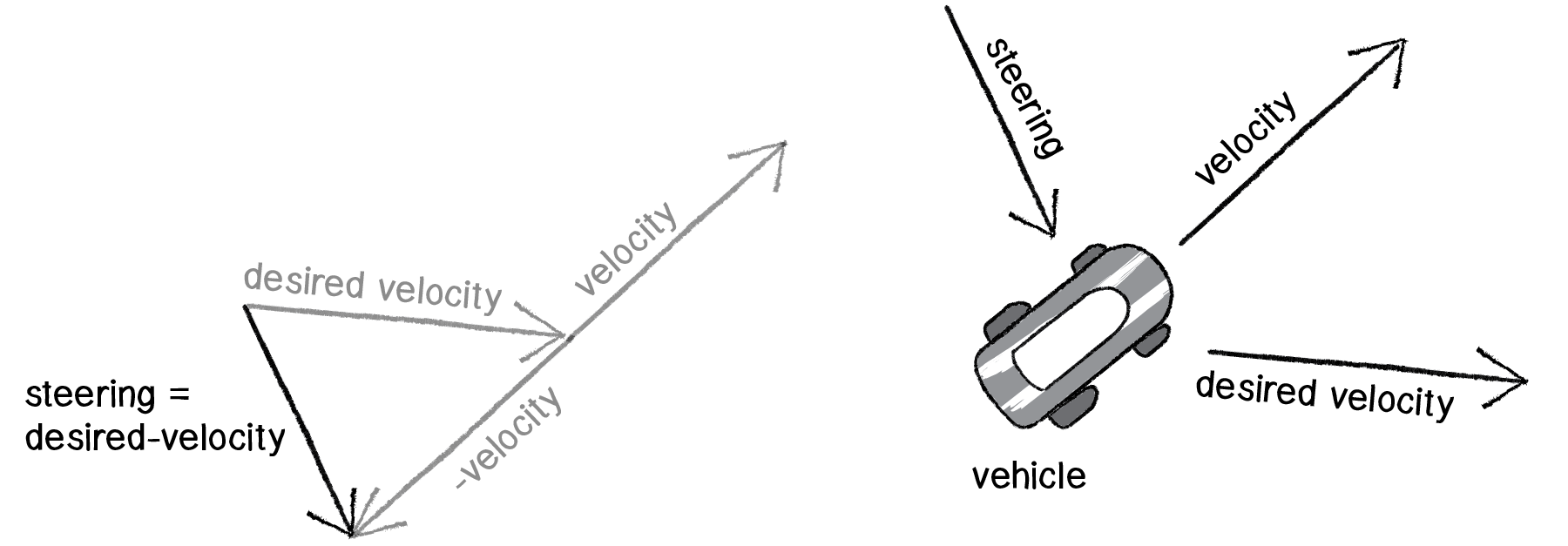
Image credit: Daniel Shiffman, The Nature of Code
Again, notice how this is not the same force as gravitational attraction. A principle of autonomous agents is that an agent has a limited ability to perceive its environment. Here is that principle, subtly embedded into Reynolds’s steering formula. If the vehicle was stationary (zero velocity), desired minus velocity, would be equal to desired. But this is not the case. The vehicle is aware of its own velocity and its steering force compensates accordingly. This creates a more active simulation, as the way in which the vehicle moves towards the targets depends on the way it is moving in the first place.
We now have a function which the Vehicle can call and pass a target location to in order to steer towards the target. However, if you look at line 7, you will notice we are calling another function called ‘applyForce()‘ which we are passing the PVector ‘steer’ to. However, we have not written an ‘applyForce()‘ function. This is because we are moving quite quickly through this lesson, so let’s quickly write this function as you will possibly be familiar with it already:
  void applyForce(PVector force) {                     // Newton’s second law: Force equals mass times acceleration.
    acceleration.add(force);                           // Acceleration is equal to the sum of all forces divided by mass
  }
Our example code, as it stands, has no feature to account for the variability in the Vehicle’s steering ability. (Is it a super sleek race car with amazing handling? Or a giant Mack truck that needs a lot of advance notice to turn?) A method to control the Steering ability can be achieved through limiting the magnitude of the steering force. Let’s call that limit the maximum force (or ‘maxForce’ for short). And so finally, we have:
class Vehicle {
  PVector location;
  PVector velocity;
  PVector acceleration;
  float maxSpeed;                    // Vehicle's top speed
  float maxForce;                    // NEW: Vehicle's maximum applied force
Followed by:
  void seek(PVector target) {
    PVector desired = PVector.sub(target, location);
    desired.normalize();
    desired.mult(maxSpeed);                            // Calculating the desired velocity to target at max speed

    PVector steer = PVector.sub(desired, velocity);    // Reynolds's formula for steering force
    steer.limit(maxForce);                             // Limit the magnitude of the steering force.

    applyForce(steer);                                 // Using our physics model we can applying the force to the object's acceleration
  }
Limiting the steering force brings up an important consideration. We must always remember that it’s not actually our goal to get the vehicle to the target as fast as possible. If that were the case, we would just say “location equals target” and there the vehicle would appear. Our goal, as Reynolds puts it, is to move the vehicle in a “lifelike and improvisational manner.” We’re trying to make it appear as if the vehicle is steering its way to the target, and so it’s up to us to play with the forces and variables of the system to simulate a given behaviour. For example, a large maximum steering force would result in a very different path than a small one. One is not inherently better or worse than the other; it depends on your desired effect. (These values need not be fixed and could change based on other conditions. Perhaps a vehicle has health: the higher the health, the better it can steer.)
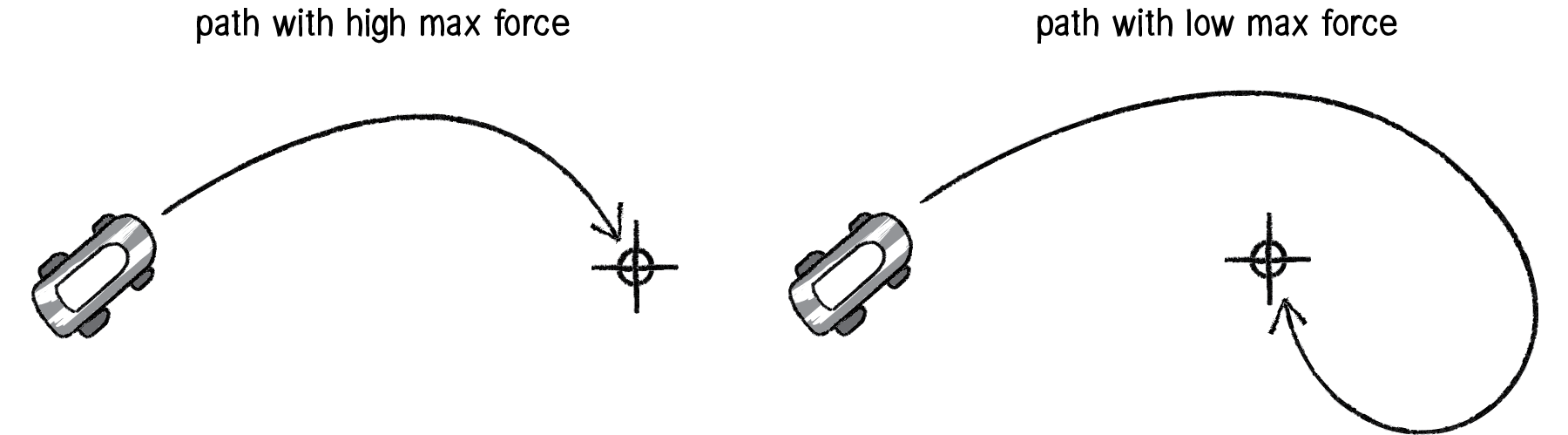
Image credit: Daniel Shiffman, The Nature of Code
Here is the full Vehicle class, incorporating the rest of the elements:
Vehicle v;

void setup() {
  size(800, 200);
  v = new Vehicle(width/2, height/2);
}

void draw() {
  background(39, 40, 34);

  PVector mouse = new PVector(mouseX, mouseY);

  // Draw an ellipse at the mouse location
  fill(255);
  noStroke();
  ellipse(mouse.x, mouse.y, 40, 40);

  // Call the appropriate steering behaviours for our agents
  v.seek(mouse);
  v.update();
  v.display();
}
class Vehicle {

  PVector location;
  PVector velocity;
  PVector acceleration;
  float r;                           // NEW: Radius of vehicle
  float maxSpeed;                    // Vehicle's top speed
  float maxForce;                    // Vehicle's maximum applied force

  Vehicle(float x, float y) {
    acceleration = new PVector(0, 0);
    velocity = new PVector(0, 0);
    location = new PVector(x, y);
    // Arbitrary values for maxspeed and force; try varying these!
    r = 6.0;
    maxSpeed = 4;
    maxForce = 0.1;
  }

  void update() {                                     // Our standard 'Euler integration' motion model
    velocity.add(acceleration);
    velocity.limit(maxSpeed);
    location.add(velocity);
    acceleration.mult(0);
  }

  void applyForce(PVector force) {                     // Newton’s second law: Force equals mass times acceleration.
    acceleration.add(force);                           // Acceleration is equal to the sum of all forces divided by mass
  }

  void seek(PVector target) {
    PVector desired = PVector.sub(target, location);
    desired.normalize();
    desired.mult(maxSpeed);                            // Calculating the desired velocity to target at max speed

    PVector steer = PVector.sub(desired, velocity);    // Reynolds's formula for steering force
    steer.limit(maxForce);                             // Limit the magnitude of the steering force.

    applyForce(steer);                                 // Using our physics model we can applying the force to the object's acceleration
  }

  void display() {
    // Vehicle is a triangle pointing in the direction of velocity
    // Since it is drawn pointing up, we rotate it an additional 90 degrees.
    float theta = velocity.heading() + PI/2;
    pushStyle();
      fill(255,0,255);
      noStroke();
      pushMatrix();
        translate(location.x,location.y);
        rotate(theta);
        beginShape();
        vertex(0, -r*2);
        vertex(-r, r*2);
        vertex(r, r*2);
        endShape(CLOSE);
      popMatrix();
    popStyle();
  }
}
3.4 Agent Flocking Behaviours
Flocking is a group animal behaviour that is a characteristic of many living creatures, such as birds, fish, and insects. In 1986, Craig Reynolds created a computer simulation of flocking behaviour and documented the algorithm in his paper, “Flocks, Herds, and Schools: A Distributed Behavioural Model.” — Daniel Shiffman
In order to demonstrate agent flocking behaviours we’ve once again had to take a quantum leap ahead of ourselves, skipping many import steps along the way, which would have provided foundation for us to better understanding of how such complex multi-agent behaviours (i.e., flocking) operate and how we would go about implementing these behaviours as code within Processing. Such steps we’ve missed include covering other simpler behaviours such as: path-following, group separation and combinations. All these behaviours a covered within The Nature of Code by Daniel Shiffman, specifically chapter 6. Autonomous Agents
Flocking is essentially the combination of three base group behaviours, each we would need to first understand and then figure out how to code:
- Cohesion — (also known as ‘centre‘): Steer towards the centre of your neighbours (stay with the group).
- Separation — (also known as ‘avoidance’): Steer to avoid colliding with your neighbours.
- Alignment— (also known as ‘copy‘): Steer in the same direction as your neighbours.

Just as we did with our separate and seek example, we’ll want our Agent objects to have a single function that manages all the above behaviours. We would call this this function ‘flock‘.
Unfortunately, the topic of agent flocking behaviours and their implementation in Processing, is far to broad and complex to be explored in it’s entirety within this workshop. Therefore, an example of 2D agent flocking is provided bellow:
/*
    * Learning Processing 3 Intermediate - Lesson 4: Autonomous Agents
 *
 * Description: Basic example of Craig Reynolds' "Flocking" behavior
 *              Rules: Cohesion, Separation, Alignment
 *              Click mouse to add boids into the system
 *
 * © Jeremy Paton (2018)
 */

Flock flock;

void setup() {
  size(900, 400);
  smooth();

  flock = new Flock();

  for (int i = 0; i < 300; i++) {              // Add an initial set of Agents into the system (200)
    Agent a = new Agent(width/2, height/2);
    flock.addAgent(a);
  }
}

void draw() {
  background(39, 40, 34);
  flock.run();
  fill(0);
}

// Add a new boid into the System
void mouseDragged() {
  flock.addAgent(new Agent(mouseX, mouseY));
}
/*
* Learning Processing 3 Intermediate - Lesson 4: Autonomous Agents
*
* Description: Flock Class - Stores an ArrayList of all the Agents
*
* © Jeremy Paton (2018)
*/
class Flock {
ArrayList agents; // An ArrayList for all the agents
Flock() {
agents = new ArrayList(); // Initialize the ArrayList
}
void run() {
for (Agent a : agents) {
a.run(agents); // Passing the entire ArrayList of agents to each agent individually
}
}
void addAgent(Agent a) {
agents.add(a);
}
} /*
* Learning Processing 3 Intermediate - Lesson 4: Autonomous Agents
*
* Description: Agent Class - Methods for Separation, Cohesion, Alignment added
*
* © Jeremy Paton (2018)
*/
class Agent {
PVector location;
PVector velocity;
PVector acceleration;
float r; // Agent size
float maxforce; // Maximum steering force
float maxspeed; // Maximum speed
color c;
// Constructor
Agent(float x, float y) {
acceleration = new PVector(0,0);
velocity = new PVector(random(-1,1),random(-1,1));
location = new PVector(x,y);
// Random initial parameters, plat with these
r = 5;
maxspeed = 2;
maxforce = 0.05;
c = color(random(120,255),random(120,255),random(120,255));
}
void run(ArrayList agents) {
flock(agents);
update();
borders();
render();
}
void applyForce(PVector force) {
// We could add mass here if we want A = F / M
acceleration.add(force);
}
// We accumulate a new acceleration each time based on three rules
void flock(ArrayList agents) {
PVector sep = separate(agents); // Separation
PVector ali = align(agents); // Alignment
PVector coh = cohesion(agents); // Cohesion
// Arbitrarily weight these forces
sep.mult(1.5);
ali.mult(0.4);
coh.mult(1.0);
// Add the force vectors to acceleration
applyForce(sep);
applyForce(ali);
applyForce(coh);
}
// Method to update location
void update() {
velocity.add(acceleration); // Update velocity
velocity.limit(maxspeed); // Limit speed
location.add(velocity);
acceleration.mult(0); // Reset accelertion to 0 each cycle
}
// A method that calculates and applies a steering force towards a target
// STEER = DESIRED MINUS VELOCITY
PVector seek(PVector target) {
PVector desired = PVector.sub(target,location); // A vector pointing from the location to the target
desired.normalize(); // Normalize desired and scale to maximum speed
desired.mult(maxspeed);
PVector steer = PVector.sub(desired,velocity); // Steering = Desired minus Velocity
steer.limit(maxforce); // Limit to maximum steering force
return steer;
}
void render() {
// Draw a triangle rotated in the direction of velocity
float theta = velocity.heading() + 3*PI/4;
fill(c);
noStroke();
pushMatrix();
translate(location.x,location.y);
rotate(theta);
rectMode(CENTER);
rect(0,0,2*r,2*r, 0,r,r,r);
popMatrix();
}
// Wraparound
void borders() {
if (location.x < -r) location.x = width+r;
if (location.y < -r) location.y = height+r;
if (location.x > width+r) location.x = -r;
if (location.y > height+r) location.y = -r;
}
// Separation
// Method checks for nearby agents and steers away
PVector separate (ArrayList agents) {
float desiredseparation = 25.0f;
PVector steer = new PVector(0,0,0);
int count = 0;
// For every Agent in the system, check if it's too close
for (Agent other : agents) {
float d = PVector.dist(location,other.location);
// If the distance is greater than 0 and less than an arbitrary amount (0 when you are yourself)
if ((d > 0) && (d < desiredseparation)) {
// Calculate vector pointing away from neighbor
PVector diff = PVector.sub(location,other.location);
diff.normalize();
diff.div(d); // Weight by distance
steer.add(diff);
count++; // Keep track of how many
}
}
// Average -- divide by how many
if (count > 0) {
steer.div((float)count);
}
// As long as the vector is greater than 0
if (steer.mag() > 0) {
// Implement Reynolds: Steering = Desired - Velocity
steer.normalize();
steer.mult(maxspeed);
steer.sub(velocity);
steer.limit(maxforce);
}
return steer;
}
// Alignment
// For every nearby boid in the system, calculate the average velocity
PVector align (ArrayList agents) {
float neighbordist = 50;
PVector sum = new PVector(0,0);
int count = 0;
for (Agent other : agents) {
float d = PVector.dist(location,other.location);
if ((d > 0) && (d < neighbordist)) {
sum.add(other.velocity);
count++;
}
}
if (count > 0) {
sum.div((float)count);
sum.normalize();
sum.mult(maxspeed);
PVector steer = PVector.sub(sum,velocity);
steer.limit(maxforce);
return steer;
} else {
return new PVector(0,0);
}
}
// Cohesion
// For the average location (i.e. center) of all nearby agents, calculate steering vector towards that location
PVector cohesion (ArrayList agents) {
float neighbordist = 50;
PVector sum = new PVector(0,0); // Start with empty vector to accumulate all locations
int count = 0;
for (Agent other : agents) {
float d = PVector.dist(location,other.location);
if ((d > 0) && (d < neighbordist)) {
sum.add(other.location); // Add location
count++;
}
}
if (count > 0) {
sum.div(count);
return seek(sum); // Steer towards the location
} else {
return new PVector(0,0);
}
}
}